Chapter 13

Continuous Systems; Waves

      Continuous String

      In Chapter 12 we examined finite systems of particles distributed along a loaded string.  A continuous string can be consider to be a limiting case of the loaded string, where we increase the number of masses n to infinity while decreasing the separation d between the masses to 0 such that (n+1)d = L = constant, and decrease the value of each mass m to 0 such that m/d = r = constant.

      Reviewing the discussion of Chapter 12 we recognize that in the limit of large n we can make the following approximations:

 

 

 

 

The displacement of the string will now become a function of x where x is the position of element j:

 

 

where

 

 

We need to keep in mind that only the real parts of our functions matter.  Assuming we know the tension in the string, the length of the string, and the mass density of the string, we can see immediately that the displacement is defined by the value of the complex amplitude.  These values are defined by specifying the displacement and the velocity of the string at time t = 0:

 

 

and

 

 

The coefficients of the amplitudes can now be found.  They key step to finding the amplitudes is to multiply each side by sin(rpx/L) where r is an integer, and integrating over x with x varying between 0 and L.  If we just focus on the sin terms we use the following relation:

 

 

Note: in the last step we have used the argument that if r ≠ s

 

 

and if r = s

 

 

 

 

 

      Example: Problem 13.2

      Rework the problem in Example 13.1 in the event that the plucked point is a distance L/3 from one end.  Comment on the nature of the allowed modes.

 

 

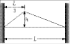
The initial conditions are

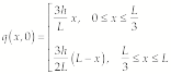                                                                                                   (1)

                                                                                                                                      (2)

Because , all of the  vanish. The  are given by

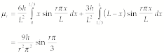                                                                         (3)

We see that  for r = 3, 6, 9, etc. The displacement function is

                         (4)

where

                                                                                                                                   (5)

The frequencies , , , etc. are absent because the initial displacement at  prevents that point from being a node. Thus, none of the harmonics with a node at  are excited.

 

 

      Energy of the String

      Since we know the displacement of the string, as function of x and t,

 

 

we can calculate the kinetic energy and the potential energy of the system.

      Consider a small segment of the string, located at x and with a width dx.  The mass of this segment is rdx.  The kinetic energy of this segment is equal to

 

 

The total kinetic energy of the string is obtained by integrating x over the entire string:

 

 

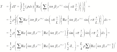
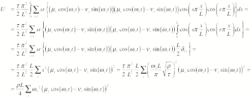
The amplitude b is a complex number with a real amplitude and an imaginary amplitude:

 

 

The kinetic energy of the string is thus equal to

 

 

In order to determine the potential energy of the system, we revisit the potential energy we determined for the loaded string in Chapter 12:

 

 

In order to approximate the a string we take the limit of n going to infinity:

 

 

In this limit, the potential energy approaches

 

 

Since the partial differential of q with respect to x is equal to

 

 

we find that the potential energy is equal to

 

The total energy of the string is

 

 

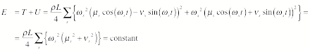
The total energy is independent of time and thus is constant.  The time-average of the kinetic energy is equal to the time-average of the potential energy:

 

 

 

 

      The Wave Equation

      In the previous sections we have looked at the possible displacement patterns of a string, based on the solution of the loaded string discussed in Chapter 12.  The solution discussed so far is appropriate for situations in which the restoring force is conservative, and no damping or driving forces are present.  In order to determine the effect of external forces on the system, we need to go back and determine the force acting on each segment of the string.

 

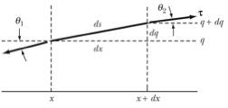
Figure 1.  Small segment of a string.

 

      Consider the segment of the string shown in Figure 1.  We assume that the tension in the string is constant, and that the tension is responsible for the restoring force that tries to bring the string back to its equilibrium position.  Consider a segment of the string of length ds.  We will assume that the parts of the string only carry out a displacement in the vertical direction.  In order to determine the restoring force, we thus need to focus on the vertical component of the tension at the end points of the section we are focusing on.  Using the geometrical information contained in Figure 1 we find that the net force is equal to

 

 

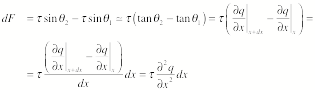
This force will result in a motion of the segment of the string.  The segment under consideration has a mass dm = r ds.  The acceleration of this section is of course related to the force acting on this section:

 

 

Combining these last two equations we obtained what is known as the wave equation:

 

 

This form of the wave equation is the "ideal" wave equation.  In order to include effects such as damping forces and driving forces, we need to include these forces in our calculation of the net force:

 

 

We can try to solve this differential equation by using the following trial solution:

 

 

Using this trial solution we can determine the various components of the equation of motion:

 

 

 

 

The equation of motion can now be rewritten as

 

 

or

 

 

We can remove the dependence on x of the left-hand side of this equation by multiplying each side by sin(spx/L) and integrating over x:

 

 

or

 

 

Our complicated second-order differential equation in x and t has been replaced by a simpler second-order differential equation in t.

 

 

      Example: Problem 3.11

      When a particular driving force is applied to a string, it is observed that the string vibration is purely in the n^th harmonic.  Find the driving force.

 

From Eq. (13.44)

                                                                                                             (1)

where  is the driving force, and  is the Fourier coefficient of the Fourier expansion of . Eq. (13.45) shows that  is the component of  effective in driving normal coordinate s. Thus, we desire  such that

                                                              

From the form of (1), we are led to try a solution of the form

                                                            

where g(t) is a function of t only.

Thus

                                                   

For n ¹ s, the integral is proportional to ; hence  for s ¹ n.

For n = s, we have

                                              

Only the  normal coordinate will be driven.

                                              

 

 

      Solving the Wave Equation

      We now return to the ideal wave equation:

 

 

Since the ratio r/t has the units of 1/(m/s)², the wave equation is frequently rewritten as

 

 

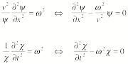
The wave equation is a second-order differential equation for a function that depends on two variables.  One approach that is frequently useful to try is separation of variables:

 

 

Substituting this expression for q into the wave equation we get

 

 

By rearranging this equation we can bring all terms that depend on x to the left-hand side and all terms that depends on t to the right-hand side:

 

 

This equation can only be correct if the term on the left-hand side is independent of x and the term on the right-hand side is independent of t.  Each term must thus be equal to the same constant, which we call w²:

 

 

These second order differential equations can be solved easily, and we find that

 

 

The general solution of the wave equation is thus

 

 

The parameter w/v is also called the wave number k.  In order to look at some of the properties of this solution, let us focus on just the first term.  Consider that we look at the displacements of the solution at (x, t).  A small time later, at time t + dt, this feature of the solution will have moved a distance dx such that:

 

 

We thus conclude that

 

 

or

 

 

The displacement we are focusing on thus appears to move with a velocity -v, and the quantity v is therefore called the wave velocity.  We note that for this solution, the solution is traveling towards the left.

      The solution is periodic and we can thus associate a wavelength with it.  We require that the amplitude at x is the same as the amplitude at x + l.  This requires that

 

 

or

 

 

The exponent of the exponential (minus the i) is called the phase of the wave.  When a particular displacement moves along the string, the associated phase will remain constant:

 

 

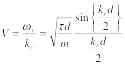
The phase velocity V is velocity of the displacement that keeps the phase constant:

 

 

Thus

 

 

We see that in general the velocities are wave-number dependent, unless w is proportional to k, and the medium is called a dispersive medium.

      Although each of the components in the general solution of the wave equation corresponds to a wave traveling either towards the left or towards the right, not all linear combinations of the solutions correspond to traveling waves.  For example consider the following linear combination of two solutions with the same amplitude:

 

 

The only component of the amplitude q that is relevant for the real world is the real part:

 

 

When we look at this real part, we see that at certain values of x the amplitude is always 0.  This solution can thus not represent a traveling wave.  This particular solution is called a standing wave.

      Up to know we have not made any constraints on the angular frequency w.  The angular frequency is a function of the wave number.  For the loaded string we found that

 

 

Based on the solutions for the loaded string we expect that the length L and the index r are related to the wavelength in the following manner:

 

 

Using this relation we can rewrite our expression for the angular frequency as follows

 

 

The phase velocity is thus equal to

 

 

For the loaded string, the index r runs from 1 to n.  The maximum value of r gives a minimum value of the wavelength:

 

 

This wavelength corresponds to the following wave number:

 

 

The corresponding frequency is thus equal to

 

 

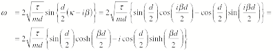
This frequency is the maximum frequency the string can support when the wave number is a real number.  The system can support larger frequencies, but at that point the wave number becomes complex.  We will now consider what the impact of a complex wave number is:

 

 

The corresponding angular frequency is

 

 

Since we are focusing on solutions of the ideal wave equation, energy must be conserved (there are no dissipative forces included) and the angular frequency must be a real number.  This implies that the imaginary part of the previous equation must be zero, or

 

 

One possibility is that b = 0, but this implies that the wave number is real, which contradicts with our initial assumption.  Thus we must require that dk/2 = p/2 or k = p/d.  In this case, we can write the angular frequency as

 

 

The dependence of the components of k on w is shown in Figure 2.

 

 

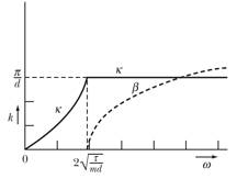
Figure 2.  Dependence of the wave number (and its components) on the angular frequency.

 

The solution of the wave equation now contains terms such as

 

 

This solution has a position-dependent amplitude, indicating that the energy of the system is localized.  However, the amplitude is not time dependent, and energy is thus conserved.