Chapter 12

Coupled Oscillations

 

      Two Coupled Harmonic Oscillators

      Consider a system of two objects of mass M.  The two objects are attached to two springs with spring constants k (see Figure 1).  The interaction force between the masses is represented by a third spring with spring constant k₁₂, which connects the two masses.

 

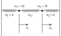
Figure 1.  Two coupled harmonic oscillators.

 

We will assume that when the masses are in their equilibrium position, the springs are also in their equilibrium positions.  The force on the left mass is equal to

 

 

The force on the right mass is equal to

 

 

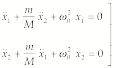
The equations of motion are thus

 

 

 

Since it is reasonable to assume that the resulting motion has an oscillatory behavior, we consider following trial functions:

 

 

 

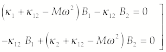
Substituting these trial functions into the equations of motion we obtain the following conditions:

 

 

 

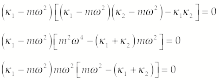
These equations only will have a non-trivial solution if

 

 

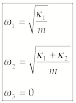
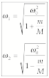
Note: the trivial solution is B₁ = B₂ = 0.  The requirement for a non-trivial solution requires that the angular frequency of the system is equal to one of the following two characteristic frequencies (the so called eigen frequencies):

 

 

 

For each of these frequencies, we can now determine the amplitudes B₁ and B₂.  Let us first consider the eigen frequency w₁.  For this frequency we obtain the following relations between B₁ and B₂:

 

 

or B₁ = -B₂.  For the eigen frequency w₂ we obtain the following relations between B₁ and B₂:

 

 

or B₁ = B₂.  The most general solution of the coupled harmonic oscillator problem is thus

 

 

 

Another approach that can be used to solve the coupled harmonic oscillator problem is to carry out a coordinate transformation that decouples the coupled equations.  Consider the two equations of motion.  If we add them together we get

 

 

If we subtract from each other we get

 

 

Based on these two equations it is clear that in order to decouple the equations of motion we need to introduce the following variables

 

 

 

The solutions to the decoupled equations of motion are

 

 

 

where the frequencies are the characteristic frequencies discussed before.  Once we have these solutions we can determine the positions of the masses as function of time:

 

 

 

We note that the solution h₁ corresponds to an asymmetric motion of the masses, while the solution h₂ corresponds to an asymmetric motion of the masses (see Figure 2).  Since higher frequencies correspond to higher energies, the asymmetric mode (out of phase) has a higher energy.

 

 

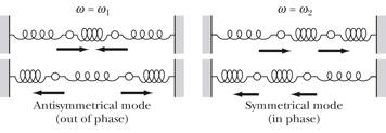
Figure 2.  Normal modes of oscillation.

 

 

      Weak Coupling

      Coupled oscillations, involving a weak coupling, are important to describe many physical systems.  For example, in many solids, the force that tie the atoms to their equilibrium positions are very much stronger than the inter-atomic coupling forces.  In the example we discussed in the pervious section, the weak coupling limit requires that k₁₂ << k.  In this approximation we can show (see text book for details) that our solutions have a high-frequency component that oscillates inside a slowly varying component (see Figure 3).  The solutions are thus sinusoidal functions with a slowly varying amplitude.

 

 

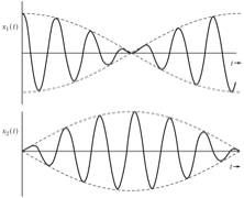
Figure 3.  Examples of solution in the weak-coupling limit.

 

 

 

      Example:  Problem 12.1

      Reconsider the problem of two coupled oscillators discussion in Section 12.2 in the event that the three springs all have different force constants.  Find the two characteristic frequencies, and compare the magnitudes with the natural frequencies of the two oscillators in the absence of coupling.

 

 

The equations of motion are

                                                                                                    (1)

We attempt a solution of the form

                                                                                                                             (2)

Substitution of (2) into (1) yields

                                                                                                (3)

In order for a non-trivial solution to exist, the determinant of coefficients of  and  must vanish. This yields

                                                                                   (4)

from which we obtain

                                                                                (5)

This result reduces to  for the case  (compare Eq. (12.7)].

If  were held fixed, the frequency of oscillation of  would be

                                                                                                                         (6)

while in the reverse case, would oscillate with the frequency

                                                                                                                         (7)

Comparing (6) and (7) with the two frequencies, and , given by (5), we find

                                        

                                                                   (8)

so that

                                                                                                                                         (9)

Similarly,

                                        

                                                                 (10)

so that

                                                                                                                                       (11)

If , then the ordering of the frequencies is

                                                                                                                     (12)

 

 

      Example:  Problem 12.3

      Two identical harmonic oscillators (with masses M and natural frequencies w0) are coupled such that by adding to the system a mass m, common to both oscillators, the equations of motion become

 

 

Solve this pair of coupled equations, and obtain the frequencies of the normal modes of the system.

 

The equations of motion are

                                                                                                                 (1)

We try solutions of the form

                                                                                                         (2)

We require a non-trivial solution (i.e., the determinant of the coefficients of  and  equal to zero), and obtain

                                                                                                             (3)

so that

                                                                                                                          (4)

and then

                                                                                                                                   (5)

Therefore, the frequencies of the normal modes are

                                                                                                                               (6)

where  corresponds to the symmetric mode and  to the anti-symmetric mode.

By inspection, one can see that the normal coordinates for this problem are the same as those for the example of Section 12.2.  Another approach to find the normal coordinates is to try to find ways to add the two equations of motion in such a way that we get an uncoupled differential equation.  Consider what happens when we multiply the first equation of motion by l and add it to the second equation of motion:

 

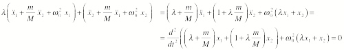
This will become an uncoupled equations if

 

 

This equation can only be correct if

 

 

and

 

 

Taking the last equation for g and substituting it into the second to last equation we obtain

 

 

This shows that

 

 

and the normal coordinates are proportional to x₂ + x₁ and x₂ - x₁.

 

 

      General Problem of Coupled Oscillations

      The results of our study of the coupled harmonic oscillator problem results in a number of different observations:

o      The coupling in a system with two degrees of freedom results in two characteristic frequencies.

o      The two characteristic frequencies in a system with two degree of freedom are pushed towards lower and higher energies compared to the non-coupled frequency.

Let us now consider a system with n coupled oscillators.  We can describe the state of this system in terms of n generalized coordinates q_i.  The configuration of the system will be described with respect to the equilibrium state of the system (at equilibrium, the generalized coordinates are 0, and the generalized velocity and acceleration are 0).  The evolution of the system can be described using Lagrange's equations:

 

 

The second term on the left-hand side will contain terms that include the generalized velocity and the generalized acceleration, and is thus equal to 0 at the equilibrium position.  Lagrange's equations thus tells us that

 

 

However, since we know how to express the kinetic energy of the system in terms of the generalized coordinates we conclude that

 

 

where

 

 

For the potential energy U we conclude that

 

 

The potential energy can be expanded around the equilibrium position using a Taylor series and we find that

 

where

 

 

We thus conclude that:

 

 

 

The equation of motion can now be written as

 

 

The index k runs over all degrees of freedom of the system, and we thus have n second order differential equations.  In order to find the general solution we try a trial solution that exhibits the expected oscillatory behavior:

 

 

With this solution, the equations of motion become

 

 

This set of equations will only has non-trivial solutions if the determinant of the coefficient must vanish:

 

 

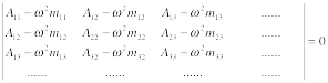
In general there will be n different values of the angular frequency.  These frequencies are called the characteristic frequencies or eigen frequencies.  Depending on the coefficients, some of the characteristic frequencies are the same (this phenomena is called degeneracy).  For each eigen frequency we can determine the ratio of the amplitudes; these amplitudes define an n-dimensional vector, also called the eigen vector.  Note: the eigen vector has a pure harmonic time dependence.

      The general solution of the system is a linear combination of the solutions q_i.  Of course, it is only the real part of the solutions that is meaningful.

      The normal coordinates can be determined by finding the appropriate linear combinations of solutions q_i that oscillates at a single frequency.  These normal coordinates are

 

 

The amplitude may be a complex number.  The normal coordinates must satisfy the following relation

 

 

Since there are n equations of motion, we also expect to see n normal coordinates, and n decoupled equations of motion.

      To illustrate the detailed steps to be followed to solve a coupled oscillator problem we will examine Example 12.4 from the textbook.  In this example, the coupled pendulum shown in Figure 4 is examined.

 

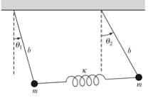
Figure 4.  Coupled pendulum of Example 12.4.

 

1.     Choose generalized coordinates.  The proper generalized coordinates in this problem are the angles q₁ and q₂.  The kinetic and the potential energy of the system can be easily expressed in terms of these angles.  We make the assumption that the spring is massless and there is thus no kinetic energy associated with the motion of the spring.  The kinetic energy of the system is thus just equal to the kinetic energy of the two masses, and thus equal to

 

 

The potential energy of the system is the sum of the potential energy associated with the change in the height of the masses and the potential energy associated with the extension or compression of the spring.  The total potential energy is thus equal to

 

 

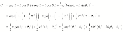
We have used the small angle approximation in order to express the sin and cos of the angles in terms of the angles.

 

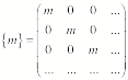
2.     Determine the A and m tensors.  In order to calculate these tensors we use the expressions for T and U obtained in step 1.  Since the kinetic energy obtained in step 1 does not contain products of the generalized velocity of mass 1 and the generalized velocity of mass 2, the mass tensor will be a diagonal tensor.  We can see this by looking at the definition of the mass tensor elements:

 

 

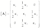
The mass tensor is thus equal to

 

 

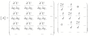
The A tensor is equal to

 

 

 

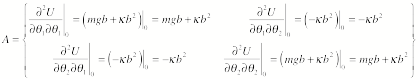
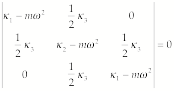
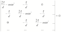
3.     Determine the eigen frequency and the eigen vectors.  The eigen frequencies can be determined by requiring that the determinant of the coefficients of the equations of motions vanishes:

 

 

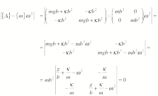
This requires that

 

 

or

 

 

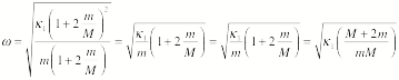
The eigen frequencies are thus equal to

 

 

 

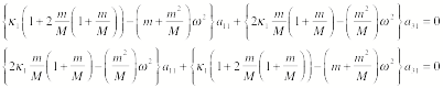
Consider the first eigen frequency.  For this frequency, the eigen vector is (a₁₁, a₂₁).  The equations of motion for this frequency are

 

 

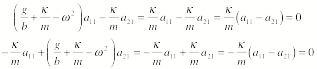
Each of these two equations tells us that a₁₁ = a₂₁.

Since the eigen vectors are orthogonal, we expect that the eigen vector for the second eigen frequency is given by a₁₂ = -a₂₂.  We come to the same conclusion if we start from the equations of motion for that frequency and the eigen vector (a₁₂, a₂₂):

 

 

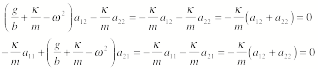
Each of these two equations tells us that a₁₂ = -a₂₂.

 

4.     Determine the scale factors required to match the initial conditions.  In this example, we do not need to match initial conditions (such as the initial displacement or the initial velocity and we thus do not need to determine scale factor).

 

5.     Determine the normal coordinates.  The normal coordinates are those coordinates that oscillate with a single frequency.  In the current example we thus observe the following normal coordinates:

 

 

 

Note: the constants in these equations need to be adjusted to match the initial conditions.

The system will carry out a motion with normal frequency 1 when h₂ = 0.  This requires that q₁ = q₂ and the motion is symmetric. The system will carry out a motion with normal frequency 2 when h₁ = 0.  This requires that q₁ = -q₂ and the motion is asymmetric.

 

 

      Molecular Vibrations

      Our theory of coupled oscillations has many important applications in molecular physics.  Each atom in a molecule has 3 degrees of freedom, and if we are looking at a molecule with n atoms, we have a total of 3n degrees of freedom.  Three different types of motion can be carried out by the atoms in the molecule: translation (3 degrees of freedom), rotation (3 degrees of freedom), and vibration (3n - 6 degrees of freedom).

      Consider a linear molecule (the equilibrium positions of all atoms are located along a straight line) with n atoms.  The number of degrees of freedom associated with Vibrational motion is 3n – 5 since there are only 2 rotational degrees of freedom.  The vibrations in a linear molecule can be longitudinal vibrations (there are n - 1 degrees of freedom associated with this type of vibrations) and transverse vibrations (there are (3n - 5) - (n - 1) = (2n - 4) degrees of freedom associated with this type of vibration).  If the vibrations are planar vibrations (the motion of all atoms is carried out in a single plane) we can specify any transverse vibration in terms of vibrations in two mutually perpendicular planes.  The characteristic frequencies in each of these planes will be the same (symmetry) and the number of characteristic frequencies will thus be equal to n - 2.

      To illustrate molecular vibrations let us consider the dynamics of a triatomic molecule (see Figure 5).

 

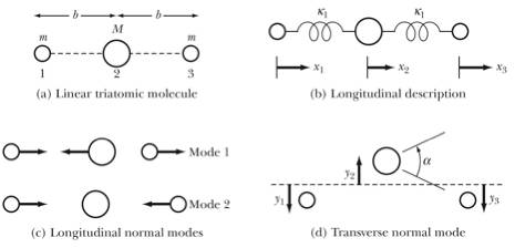
Figure 5.  Vibrational motion of a linear triatomic molecule.

 

In order to determine the vibrational modes of this system we look at the longitudinal and transversal modes separately.  Since we are not interested in pure translational motion we can require that the center of mass of the system is at rest.  This means that we do not have 3 independent position coordinates, but only 2.  For example, we can eliminate the position of the heavy atom:

 

 

In order to determine the normal modes, we will follow the same procedure as we used in the previous example (note: this differs from the approach used in the textbook).

 

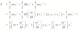
1.     Choose generalized coordinates.  The proper generalized coordinates in this problem are the displacements x₁ and x₂.  The kinetic and the potential energy of the system can be easily expressed in terms of these displacements.  The kinetic energy of the system is thus just equal to the kinetic energy of the three atoms, and thus equal to

 

 

The potential energy of the system is the sum of the potential energy associated with the compression of the springs.  The total potential energy is thus equal to

 

 

 

2.     Determine the A and m tensors.  In order to calculate these tensors we use the expressions for T and U obtained in step 1.  Since the kinetic energy obtained in step 1 does not contain products of the generalized velocity of mass 1 and the generalized velocity of mass 2, the mass tensor will be a diagonal tensor.  We can see this by looking at the definition of the mass tensor elements:

 

 

The mass tensor is thus equal to

 

 

The A tensor is equal to

 

 

 

3.     Determine the eigen frequency and the eigen vectors.  The eigen frequencies can be determined by requiring that the determinant of the coefficients of the equations of motions vanishes:

 

This requires that

 

 

or

 

 

Consider the two signs.  First the positive sign:

 

 

This is equivalent to

 

 

or

 

 

Now consider the negative sign:

 

 

This is equivalent to

 

or

 

 

Consider the first eigen frequency, and assume the corresponding eigen vector is (a₁₁, a₂₁).  The equations of motion for this frequency are

 

 

Substituting the expression of the first eigen frequency in these equations we obtain for each equation the following expression:

 

 

This equations tells us that a₁₁ = -a₃₁.  Since the eigen vectors are orthogonal, we expect that the eigen vector for the second eigen frequency is given by a₁₂ = a₃₂.

 

4.     Determine the scale factors required to match the initial conditions.  In this example, we do not need to match initial conditions (such as the initial displacement or the initial velocity and we thus do not need to determine scale factor).

 

5.     Determine the normal coordinates.  The normal coordinates are those coordinates that oscillate with a single frequency.  In the current example we thus observe the following normal coordinates:

 

 

 

Note: the constants in these equations need to be adjusted to match the initial conditions.

The system will carry out a motion with normal frequency 1 when h₂ = 0.  This requires that x₁ = -x₃ and the motion is asymmetric. The system will carry out a motion with normal frequency 2 when h₁ = 0.  This requires that x₁ = x₃ and the motion is symmetric.

Note: the normal frequency 1 is equal to the frequency of a mass m on a spring whose other end remains fixed.  This mode requires the central atom to remain fixed, and this can be achieved when the motion is asymmetric since the forces exerted by the two springs on the central mass cancel.

 

The transverse vibration of the molecule can be specified in terms of a single parameter a.  For this mode of vibration we will get a single "uncoupled" differential equation with a single corresponding characteristic frequency.  The calculation of this frequency is shown in detail in the text book and will not be reproduced here.

 

 

      Example:  Problem 12.21

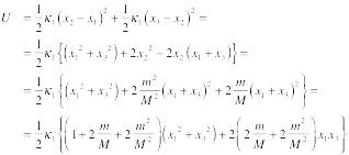
      Three oscillators of equal mass m are coupled such that the potential energy of the system is given by

 

 

where

 

 

Find the eigen frequencies by solving the secular equation.  What is the physical interpretation of the zero-frequency mode?

 

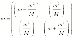
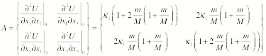
The tensors  and  are:

                                                                                                             (1)

                                                                                                                         (2)

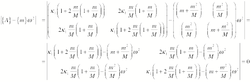
thus, the secular determinant is

                                                                                             (3)

from which

                                                                               (4)

In order to find the roots of this equation, we first set  and then factor:

                                                                               (5)

Therefore, the roots are

                                                                                                                              (6)

Consider the case . The equation of motion is

                                                                                                                                 (7)

so that

                                                                                                                                             (8)

with the solution

                                                                                                                                  (9)

That is, the zero-frequency mode corresponds to a translation of the system with oscillation.

 

 

      The Loaded String

      A good model of an elastic string is a string of particles of mass m, each separated by a distance d (see Figures 6 and 7).  We will assume that the tension in the string is constant and equal to t.

 

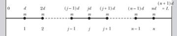
Figure 6.  The loaded string.

 

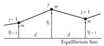
Figure 7.  Calculation of the restoring force acting on mass j.

 

In examining this problem, we will make the following assumptions:

·      The masses can only move in the vertical direction (thus only the component of the tension in the vertical direction matters).

·      The potential energy of the system is the potential energy associated with the tension in the string.

·      We assume that the displacements from the equilibrium positions are small.

·      We ignore the gravitational forces acting on the masses (and the associated gravitational potential energy).

In order to calculate the force acting on mass j we calculate the vertical components due to the tension in the left and right section of the string:

 

 

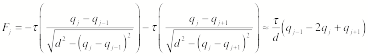
In the last step we have made the assumption that the vertical displacement is small compared to the distance d. Since the force on mass j depends not only on the position of mass j but also on the position of masses j - 1 and j + 1.  We can use the force on the n masses to obtain n coupled differential equations that we can try to solve.  Consider the following trial function:

 

 

Substituting this function into our differential equation we obtain

 

 

or

 

 

The amplitudes a can be complex.  Based on the type of motion we expect the system to carry out, we can try to parameterize the amplitude dependence on j in the following way:

 

 

where a is now a real number.  Taking this expression for a_j and substituting it into the previous equation we obtain

 

 

This expression can be used to find the following expression for the angular frequency:

 

 

or

 

 

Since there must be n eigen frequencies, we expect to find n distinct values of g.

      Additional constraints are imposed on the solution by requiring that the boundary conditions are met:

·      a₀ = 0:  This condition requires that (note: we only consider the real part of the amplitude)

 

 

or

 

 

·      a_n+1 = 0:  This condition requires that

 

 

The argument of the sin function must thus be an integer multiple of p:

 

 

or

 

 

where s = 1, 2, 3, …, n.

Since the boundary conditions provide us with n different values of the parameter g, we expect that there will also be n unique values of the angular frequency for this system:

 

 

where s = 1, 2, 3, …, n.

      Putting all the different pieces of information together we can now write down the general solution of the loaded string problem:

 

 

and

 

 

      We can also use the Lagrangian method to find the normal modes of the system, but as we will see, this approach is much less transparent than the approach just used.  In order to apply this procedure we need to determine the kinetic energy and the potential of the system in terms of the generalized coordinates.  In this particular problem, the best choice for the generalized coordinates is the vertical displacement of the masses.  In terms of these displacements we can write the kinetic energy as

 

 

In order to determine the potential energy of the system, we first have to determine the potential energy of mass j.  Since we know the relation between the potential energy and the force, we can see that the potential energy is equal to

 

 

Note: the index runs from j = 1 to j = n + 1.  There are no masses at position 0 and at position (n+1)d; these positions are the ends of the string.  The displacement at these locations is equal to 0.

Note: in order to verify that the potential energy is correct, we need to show that its gradient is related to the force on mass j:

 

The mass tensor m for the system is given by

 

 

The potential tensor A for the system is given by

 

 

The eigen frequencies can now be found by requiring that the secular determinant is equal to 0:

 

 

We can solve this equation for w but the results are more difficult to interpret than the results obtained with out first approach.