Chapter 11
Dynamics of Rigid Bodies
A rigid body is a collection of particles with fixed relative positions, independent of the motion carried out by the body. The dynamics of a rigid body has been discussed in our introductory courses, and the techniques discussed in these courses allow us to solve many problems in which the motion can be reduced to two-dimensional motion. In this special case, we found that the angular momentum associated with the rotation of the rigid object is directed in the same direction as the angular velocity:
![]()
In this equation, I is the moment of inertia of the rigid body which was defined as
![]()
where ri is the distance of mass mi from the rotation axis. We also found that the kinetic energy of the body, associated with its rotation, is equal to
![]()
The complexity of the motion increases when we need three dimensions to describe the motion. There are many different ways to describe motion in three dimensions. One common method is to describe the motion of the center of mass (in a fixed coordinate system) and to describe the motion of the components around the center of mass (in the rotating coordinate system).
The Inertia Tensor
In Chapter 10 we derived the following relation between the velocity of a particle in the fixed reference frame, vf, and its velocity in the rotating reference frame vr:
![]()
If we assume that the rotating frame is fixed to the rigid body, then vr = 0.
The total kinetic energy of the rigid body is the sum of the kinetic energies of each component of the rigid body. Thus
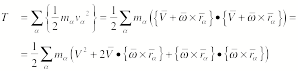
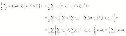
Let us now examine the three terms in this expression:
![]()
![]()
The second term is zero, if we
choose the origin of the rotating coordinate system to coincide with the center
of mass of the rigid object.
Using
the previous expressions, we can now rewrite the total kinetic energy of the
rigid object as
![]()
The quantity Iij is called the inertia tensor,
and is a 3 x 3 matrix:

Based on the definition of the
inertia tensor we make the following observations:
·
The
tensor is symmetric: Iij = Iji. Of the 9 parameters, only 6 are free parameters.
·
The
non-diagonal tensor elements are called products of inertia.
·
The
diagonal tensor elements are the moments of inertia with respect to the three
coordinate axes of the rotating frame.
Angular
Momentum
The
total angular momentum L of the rotating
rigid object is equal to the vector sum of the angular momenta of each
component of the rigid object. The
ith component of L is
equal to

This equation clearly shows that the
angular momentum is in general not parallel to the angular velocity. An example of a system where the
angular momentum is directed in a different from the angular velocity is shown
in Figure 1.
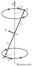
Figure 1. A rotating dumbbell is an example of a
system in which the angular velocity is not parallel to the angular momentum.
The rotational kinetic energy can
also be rewritten in terms of the angular momentum:
![]()
Principal
Axes
We
always have the freedom to choose our coordinate axes such that the problem we
are trying solve is simplified. When we are working on problems that involve the use of the inertia
tensor, we can obtain a significant simplification if we can choose our
coordinate axes such that the non-diagonal elements are 0. In this case, the inertia tensor would
be equal to

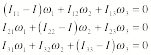
For this inertia tensor we get the
following relation between the angular momentum and the angular velocity:
![]()
The rotational kinetic energy is
equal to
![]()
The axes for which the non-diagonal
matrix elements vanish are called the principal axes of inertia.
The
biggest problem we are facing is how do we determine the proper coordinate
axes? If the angular velocity
vector is directed along one of the three coordinate axes that would get rid of
the non-diagonal inertia tensor elements, we expect to see the following
relation between the angular velocity vector and the angular momentum:
![]()
Substituting the general form of the
inertia tensor into this expression, we must require that

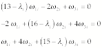
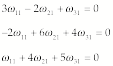
This set of equations can be
rewritten as
This set of equations only has a
non-trivial solution if the determinant of the coefficients vanish. This requires that

This requirement leads to three
possible values of I. Each of these corresponds to the moment
of inertia about one of the principal aces.
Example:
Problem 11.13
A
three-particle system consists of masses mi and coordinates (x1, x2, x3) as follows:
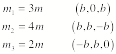
Find the inertia tensor, the
principal axes, and the principal moments of inertia.
We get
the elements of the inertia tensor from Eq. 11.13a:

Likewise
![]() and
and
![]()

Likewise
![]()
and
![]()
Thus the
inertia tensor is
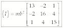
The
principal moments of inertia are
gotten by solving
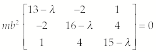
Expanding
the determinant gives a cubic equation in l:
![]()
Solving
numerically gives


To find the
principal axes, we substitute into (see example 11.3):
For i = 1, we have
![]()
Solving the
first for
![]() and substituting into the second gives
and substituting into the second gives
![]()
Substituting
into the third now gives
![]()
or
![]()
So, the
principal axis associated with
![]() is
is
![]()
Proceeding
in the same way gives the other two principal axes:
![]()
We note that the principal axes are
mutually orthogonal, as they must be.
Our
observation in problem 11.13 that the principal vectors are orthogonal is true
in general. We can prove this in
the following manner. For the mth principal moment the following relations must hold:
![]()
![]()
Combining these two equations we
obtain
![]()
Now multiply both sides of this
equation by win and
sum over i:
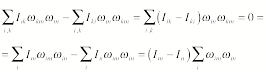
![]()
A similar relation can be obtained
for the nth principal moment, multiplied by wkm and summed over k:
![]()
If we subtract the last equation
from the one-before-last equation we obtain the following result:
Assuming that the principal momenta
are distinct, the previous equation can only be correct if
![]()
which shows the principal axes are
orthogonal.
Transformations
of the Inertia Tensor
In
our discussion so far we have assumed that the origin of the rotating reference
frame coincidence with the center of mass of the rigid object. In this Section we will examine what
will change if we do not make this assumption.
Consider
the two coordinate systems shown in Figure 2. One reference frame, the x frame, has its origin O coincide with the center of mass of the rigid object; the second reference
frame, the X frame, has an origin Q that is displaced with respect
to the center of mass of the rigid object.
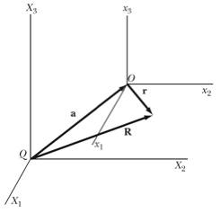
Figure 2. Two
coordinate systems used to describe our rigid body.
The inertia tensor Jij in reference frame X is defined in the same way as it was defined
previously:
![]()
The coordinates in the X frame are related to the coordinates in the x frame in the following way:
![]()
Using this relation we can express
the inertia tensor in reference frame X in terms of the coordinates in reference frame x:

The last term on the right-hand side
is equal to 0 since the origin of the coordinate system x coincides with the center of mass of the object:
![]()
The relation between the inertia
tensor in reference frame X and the
inertia tensor in reference frame x is thus given by
![]()
This relation is called the Steiner's
parallel-axis theorem and is one example
of how coordinate transformations affect the inertia tensor.
The
transformation discussed so far is a simple translation. Other important transformations are
rotations. In Chapter 1 we
discussed many examples of rotations, and determined that the most general way
to express rotations is by using the rotation matrix l:
![]()
Since this transformation rule is
valid for vectors in general, the same rule can be used to describe the
transformation of the angular momentum and angular velocity vectors:
![]()
![]()
In order to determine the relation
between the inertia tensor in the two coordinate frames, we use the fact that
the angular momentum is the product of the inertia tensor and the angular
velocity, in both frames:
![]()
and
![]()
In order
to relate the inertia tensors, we use the coordinate transformations for L and w:
![]()
This equation can be simplified if
we multiply each side by lik and sum over k:
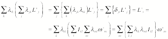
where we have used the orthogonal
properties of the rotation matrix. Using the relation between the angular momentum and the angular velocity
in the rotated coordinate frame we see that the inertia tensors in the two
coordinate frames are related as follows:
![]()
where lt is the transposed matrix. In
tensor notation we can rewrite this relation as
![]()
It turns out that for any inertia
tensor we can find a rotation such that the inertia tensor in the rotated frame
is a diagonal matrix (all non-diagonal elements are equal to 0).
We
thus have seen two different approaches to diagonalize the inertia tensor: 1)
find the principal axes of inertia, and 2) find the proper rotation matrix.
Example:
Problem 11.16
Consider
the following inertia tensor:
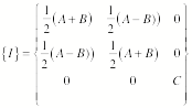
Perform a rotation of the coordinate
system by an angle q about the x3 axis. Evaluate the transformed tensor elements, and show that the
choice q = p/4 renders the inertia tensor
diagonal with elements A, B, and C.
The
rotation matrix is
 (1)
(1)
The moment
of inertia tensor transforms according to
![]() (2)
(2)
That is

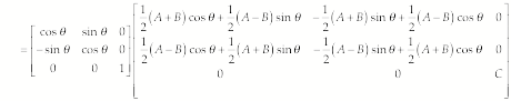

or
 (3)
(3)
If
![]() ,
,
![]() . Then,
. Then,
 (4)
(4)
Euler
Angles
Any
rotation between different coordinate systems can be expressed in terms of
three successive rotations around the coordinate axes. When we consider the transformation
from the fixed coordinate system x' to
the body coordinate system x, we
call the three angles the Euler angles f, q, and y (see Figure 3).

Figure 3. The Euler angles used to transform the
fixed coordinate system x' into the body
coordinate system x.
The total transformation matrix is
the product of the individual transformations (note order)

With each of the three rotations we
can associate an angular velocity w. To express the angular velocity in the
body coordinate system, we can use Figure 3c.
·
wf: Figure 3c shows that the angular
velocity wf is directed in the x2''' - x3''' plane. Its projection along the x3''' axis, which is also the x3 axis, is equal to
![]()
The projection
along the x2''' axis is equal
to
![]()
Figure 3c shows
that when we project this projection along the x1 and x2 axes we obtain the following components in the body coordinate system:
![]()
![]()
·
wq: Figure 3c shows that the angular
velocity wq is directed in the x1''' - x2''' plane. Its projection along the x3''' axis, which is also the x3 axis, is equal to 0.
![]()
Figure 3c shows
that when we project wq along the x1 and x2 axes we obtain the following components
in the body coordinate system:
![]()
![]()
·
wy: Figure 3c shows that the angular
velocity wy is directed along the x3''' axis, which is also the x3 axis. The components along the other body axes are 0. Thus:
![]()
![]()
![]()
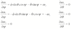
The angular velocity, in the body
frame, is thus equal to
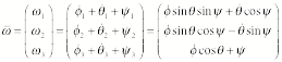
The
Force-Free Euler Equations
Let's
assume for the moment that the coordinate axis correspond to the principal axes
of the body. In that case, we can
write the kinetic energy of the body in the following manner:
![]()
where Ii are the principal moments of the rigid
body. If for now we consider that
the rigid object is carrying out a force-free motion (U = 0) then the Lagrangian L will be equal to the kinetic energy T. The
motion of the object can be described in terms of the Euler angles, which can
serve as the generalized coordinates of the motion. Consider the three equations of motion for the three
generalized coordinates:
·
The
Euler angle f: Lagrange's equation for the coordinate f is
![]()
Differentiating the
angular velocity with respect to the coordinate f we find
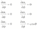
and Lagrange's
equation becomes
![]()
·
The
Euler angle q: Lagrange's equation for the coordinate q is
![]()
Differentiating the
angular velocity with respect to the coordinate q we find

and Lagrange's
equation becomes
![]()
·
The
Euler angle y: Lagrange's equation for the coordinate y is
![]()
Differentiating the
angular velocity with respect to the coordinate y we find
and Lagrange's
equation becomes
![]()
Of all three equations of motion, the
last one is the only one to contain just the components of the angular velocity. Since our choice of the x3 axis was arbitrary, we expect that
similar relations should exist for the other two axes. The set of three equation we obtain in
this way are called the Euler equations:
![]()
![]()
![]()
As
an example of how we use Euler's equations, consider a symmetric top. The top will have two different
principal moments: I1 = I2 and I3. In this case, the first Euler equations reduces to
![]()
or
![]()
The other two Euler equations can be
rewritten as
![]()
![]()
This set of equations has the
following solution:
![]()
![]()
The magnitude of the angular
velocity of the system is constant since
![]()
The angular velocity vector traces
out a cone in the body frame (it precesses around the x3 axis - see Figure 4). The rate with which the angular
velocity vector precesses around the x3 axis is determined by the value of W. When the principal moment I3 and the principal moment I1 are similar, W will become very small.
Since
we have assumed that there are no external forces and torques acting on the
system, the angular momentum of the system will be constant in the fixed
reference frame. If the angular
momentum is initially pointing along the x'3 axis it will continue to point along this axis (see Figure 5). Since there are no external forces and
torques acting on the system, the rotation kinetic energy of the system must be
constant. Thus
![]()
Since the angle between the angular
velocity vector and the angular momentum vector must be constant, the angular
velocity vector must trace out a space cone around the x'3 (see Figure 5).
|
|
Figure 4. The angular velocity of a force-free
symmetric top, precessing around the x3 axis in the body frame.
|
Figure 5. The
angular velocity of a force-free symmetric top, tracing out a space-cone
around the x'3 axis in the
body frame.
|
Example:
Problem 11.27
A
symmetric body moves without the influence of forces or torques. Let x3 be the symmetry axis of the body and L be along x3'. The angle
between the angular velocity vector and x3 is a. Let w and L initially be in the x2-x3 plane. What
is the angular velocity of the symmetry axis about L in terms of I1, I3, w, and a?

Initially:

Thus
![]() (1)
(1)
From Eq. (11.102)
![]()
Since
![]() , we have
, we have
![]() (2)
(2)
From Eq. (11.131)
![]()
(2) becomes
![]() (3)
(3)
From (1), we may construct the following triangle

from which
![]()
Substituting into (3) gives
![]()
The
Euler Equations in a Force Field
When
the external forces and torques acting on the system are not equal to 0, we can
not use the method we have used in the previous section to obtain expressions
for the angular velocity and acceleration. The procedure used in the previous section relied on the
fact that the potential energy U is 0 in
a force-free environment, and therefore, the Lagrangian L is equal to the kinetic energy T.
When
the external forces and torques are not equal to 0, the angular momentum of the
system is not conserved:
![]()
Note that this relation only holds
in the fixed reference frame since this is the only good inertial reference
frame. In Chapter 10 we looked at
the relation between parameters specified in the fixed reference frame compared
to parameters specified in the rotating reference frame, and we can use this
relation to correlate the rate of change of the angular momentum vector in the
fixed reference frame with the rate of change of the angular momentum vector in
the rotating reference frame:
![]()
This relation can be used to
generate three separate relations by projecting the vectors along the three
body axes:
![]()
![]()
![]()
These equations are the Euler
equations for the motion of the rigid body in a force field. In the absence of a torque, these
equations reduce to the force-free Euler equations.
Example:
Motion of a Symmetric Top with One Point Fixed
In
order to describe the motion of a top, which has its tip fixed, we use two
coordinate systems whose origins coincide (see Figure 6). Since the origins coincide, the
transformation between coordinate systems can be described in terms of the
Euler angles, and the equations of motion will be the Euler equations:
![]()
![]()
![]()
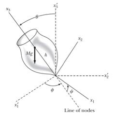
Figure 6. Spinning top with fixed tip.
Since the top is symmetric around
the x3 axis, it principal
moments of inertia with respect to the x1 and x2 axes are identical. The Euler
equations now become
![]()
![]()
![]()
The first equation immediately tells
us that
![]()
The motion of the top is often
described in terms of the motion of its rotating axes. The kinetic energy of the system is
equal to
![]()
The potential energy of the system,
assuming the center of mass of the top is located a distance h from the tip, is equal to
![]()
The Lagrangian is thus equal to
![]()
The Lagrangian does not depend on f and y,
and thus
![]()
![]()
We thus conclude that the angular
momenta associated with the Euler angles f and y are constant:
![]()
![]()
Expressing the momenta in terms of
the Euler angles f and y allows us to express the rate of
change of these Euler angles in terms of the angular momenta:
![]()
![]()
Since there are no non-conservative
forces acting on the top, the total energy E of the system is conserved. Thus
![]()
The total energy can be rewritten in
terms of the angular momenta:

Since the angular velocity with
respect to the x3 axis is constant, we
can subtract it from the energy E to get the effective energy E'
(note: this is equivalent to choosing the zero point of the energy scale). Thus
![]()
The effective energy only depends on
the angle q and on dq/dt since the angular momenta are constants. The manipulations we have carried out have reduced the
three-dimensional problem to a one-dimensional problem. The first term in the effective energy
is the kinetic energy associated with the rotation around the x1 axis. The last two terms depend only on the angle q and not on the angular velocity dq/dt. These terms are what we
could call the effective potential energy, defined as
![]()
The effective potential becomes
large when the angle approaches 0 and p. The angular dependence of the effective
potential is shown in Figure 7. If
the total effective energy of the system is E1', we expect the angle q to vary between q1 and q2. We thus expect that the angle of
inclination of the top will vary between these two extremes.
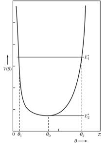
Figure 7. The
effective potential of a rotating top.
The
minimum effective energy that the system can have is E2'. The corresponding angle can be found by requiring
![]()
This requirement can be rewritten as
a quadratic equation of a parameter b,
where b is defined as
![]()
In general, there are two solutions
to this quadratic equation. Since b is a real number, the solution must
be real, and this requires that
![]()
This equation can be rewritten as
![]()
When we study a spinning top, the
spin axis is oriented such that q0 < p/2. The previous equation can then be
rewritten as
![]()
or
![]()
There is thus a minimum angular
velocity the system must have in order to produce stable precession. The rate of precession can be found by
calculating
![]()
Since b has two possible values, we expect to see two different precession rates: one
resulting in fast precession, and one resulting in slow precession.
When
the angle of inclination is not equal to q0,
the system will oscillate between two limiting values of q. The precession rate will be a function of q and can vary between positive and negative
values, depending on the values of the angular momenta. The phenomenon is called nutation, and
possible nutation patterns are shown in Figure 8. The type of nutation depends on the initial conditions.
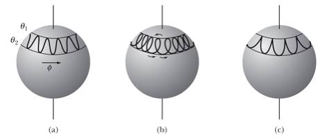
Figure 8. The
nutation of a rotating top.
Example:
Problem 11.30
Investigate
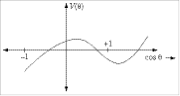
the equation for the turning points of the nutational motion by setting dq/dt = 0 in the equation of the effective energy. Show that the resulting equation is cubic in cosq and has two real roots and one
imaginary root.
If we set
![]() in the equation for the effective energy we obtain
in the equation for the effective energy we obtain
![]() (1)
(1)
Re-arranging, this equation can be written as
![]() (2)
(2)
which is cubic in cosq.
V(q)
has the form shown in the diagram. Two of the roots occur in the region
![]() , and one root lies outside this range and is therefore
imaginary.
, and one root lies outside this range and is therefore
imaginary.
Stability
of Rigid-Body Rotations
The
rotation of a rigid body is stable if the system, when perturbed from its
equilibrium condition, carries out small oscillations about it. Consider we use the principal axes of
rotation to describe the motion, and we choose these axes such that I3 > I2 > I1. If the system rotates around the x1 axis we can write the angular velocity vector as
![]()
Consider what happens when we apply a small perturbation
around the other two principal axes such that the angular velocity becomes
![]()
The corresponding Euler equations are
![]()
![]()
![]()
Since we are talking about small
perturbations from the equilibrium state, lm will be small and can be set to 0. The second equation can thus be used to conclude that
![]()
The remaining equations can be rewritten as
![]()
![]()
The last equation can be differentiated to obtain
![]()
The term within the parenthesis is positive since we assumed
that I3 > I2 > I1. This differential equation has the following solution:
![]()
where
![]()
When we look at the perturbation around the x3 axis we find the following differential
equation
![]()
The solution of the second-order differential equation is
![]()
We see that the perturbations around the x2 axis and the x3 axis oscillate around the equilibrium
values of l = m = 0. We thus conclude that the rotation around the x1 axis is stable.
Similar
calculations can be done for rotations around the x2 axis and the x3 axis. The perturbation frequencies obtained in those cases are
equal to
![]()
![]()
We see that the first frequency is an imaginary number while
the second frequency is a real number. Thus, the rotation around the x3 axis is stable, but the rotation around the x2 axis is unstable.
Example:
Problem 11.34
Consider
a symmetrical rigid body rotating freely about its center of mass. A frictional torque (Nf = -bw) acts to slow down the
rotation. Find the component of
the angular velocity along the symmetry axis as a function of time.
The Euler equation, which describes the rotation of an object about its symmetry axis, say the x axis, is
![]()
where
![]() is the component
of torque along Ox. Because the object is symmetric about
the x axis, we have
is the component
of torque along Ox. Because the object is symmetric about
the x axis, we have
![]() , and the above
equation becomes
, and the above
equation becomes
![]()

In this Chapter we focus on the dynamics of rigid bodies.
In our introductory courses the motion of the rigid body is reduced to a two-dimensional problem. In this Chapter we will descibe the motion of a rigid body in three dimensions.

