Chapter 9

Dynamics of a System of Particles

 

      The Center-of-Mass

      As we discussed in Chapter 9, it is often useful to separate the motion of a system into the motion of its center of mass and the motion of its component relative to the center of mass.  The definition of the position of the center of mass for a multi-particle system (see Figure 1) is similar to its definition for a two-body system:

 

 

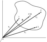
Figure 1.  The location of the center of mass of a multi-particle system.

 

If the mass distribution is a continuous distribution, the summation is replaced by an integration:

 

 

 

 

      Example: Problem 9.1

      Find the center of mass of a hemispherical shell of constant density and inner radius r₁ and outer radius r₂.

 

      Put the shell in the z > 0 region, with the base in the x-y plane.  By symmetry,

 

 

To find the z coordinate of the center-of-mass we divide the shell into thin slices, parallel to the xy plane.

 

 

Using z = r cosq and doing the integrals gives

 

 

 

 

      Linear Momentum

      Consider a system of particles, of total mass M, exposed to internal and external forces.  The linear momentum for this system is defined as

 

 

The change in the linear momentum of the system can be expressed in terms of the forces acting on all the particles that make up the system:

 

 

We see that the linear momentum is constant if the net external force acting on the system is 0 N.  If there is an external force acting on the system, the component of the linear momentum in the direction of the net external force is not conserved, but the components in the directions perpendicular to the direction of the net external force are conserved.

We conclude that the linear momentum of the system has the following properties:

 

1.     The center of mass of a system moves as if it were a single particle with a mass equal to the total mass of the system, M, acted on by the total external force, and independent of the nature of the internal forces.

 

2.     The linear momentum of a system of particles is the same as that of a single particle of mass M, located at the position of the center of mass, and moving in the manner the center of mass is moving.

 

3.     The total linear momentum for a system free of external forces is constant and equal to the linear momentum of the center of mass.

 

 

      Angular Momentum

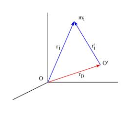
      Consider a system of particles that are distributed as shown in Figure 2.  We can specify the location of the center of mass of this system by specifying the vector R.  This position vector may be time dependent.  The location of each component of this system can be specified by either specifying the position vector, r_a, with respect to the origin of the coordinate system, or by specifying the position of the component with respect to the center of mass, r_a'.

 

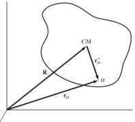
Figure 2.  Coordinate system used to describe a system of particles.

 

The angular momentum of this system with respect to the origin of the coordinate system is equal to

 

 

Since

 

 

we can rewrite the expression for the angular momentum as

 

 

The angular momentum is thus equal to sum of the angular momentum of the center of mass and the angular momentum of the system with respect to the center of mass.

      The rate of change in the angular momentum of the system can be determined by using the following relation:

 

 

For the system we are currently discussing we can thus conclude that

 

 

The last step in this derivation is only correct of the internal force between i and j is parallel or anti-parallel to the relative position vector, but this was one of the two assumptions we made about the internal forces at the beginning of this Chapter.  Since the vector product between the position vector and the force vector is the torque N associated with this force, we can rewrite the rate of change of the angular momentum of the system as

 

 

We conclude that the angular momentum of the system has the following properties:

 

1.     The total angular momentum about an origin is the sum of the angular momentum of the center of mass about that origin and the angular momentum of the system about the position of the center of mass.

 

2.     If the net resultant torques about a given axis vanish, then the total angular momentum of the system about that axis remained constant in time.

 

3.     The total internal torque must vanish if the internal forces are central, and the angular momentum of an isolated system can not be altered without the application of external forces.

 

 

      Example: Problem 9.13

      Even though the total force on a system of particles is zero, the net torque may not be zero.  Show that the net torque has the same value in any coordinate system.

 

The total force acting on the system can be rewritten in terms of the external and internal forces:

 

 

The problem states that the total force is equal to zero.

Now consider two coordinate systems with origins at 0 and 0¢

 

where

                                                 is a vector from 0 to 0¢

                                                 is the position vector of m_i in 0

                                                 is the position vector of m_i in 0¢

We see that .  The torque with respect to 0 is given by

 

 

The torque with respect to 0¢ is equal to

 

 

But, since it is given that

 

 

we conclude that

 

 

 

 

      Energy

      The total energy of a system of particles is equal to the sum of the kinetic and the potential energy.

      The kinetic energy of the system is equal to the sum of the kinetic energy of each of the components.  The kinetic energy of particle i can either be expressed in terms of its velocity with respect to the origin of the coordinate system, or in terms of its velocity with respect to the center of mass:

 

 

The kinetic energy of the system is thus equal to

 

 

Based on the definition of the position of the center of mass:

 

 

we conclude that

 

 

The kinetic energy of the system is thus equal to

 

 

The change in the potential energy of the system when it moves from a configuration 1 to a configuration 2 is related to the work done by the forces acting on the system:

 

 

If we make the assumption that the forces, both internal and external, are derivable from potential functions, we can rewrite this expression as

 

 

The first term on the right-hand side can be evaluated easily:

 

 

The second term can be rewritten as

 

 

Here we have used the fact that the internal force between i and j satisfy the following relation

 

 

and thus

 

 

The integral can be evaluated easily:

 

 

The total potential energy of the system U is defined as the sum of the internal and the external potential energy and is equal to

 

 

The work done by al the force to make the transition from configuration 1 to configuration 2 is

 

 

Using the work-energy theorem we can conclude that

 

 

or

 

 

We thus see that the total energy is conserved.  If the system of particles is a rigid object, the components of the system will retain their relative positions, and the internal potential energy of the system will remain constant.

We conclude that the total energy of the system has the following properties:

 

1.     The total kinetic energy of the system is equal to the sum of the kinetic energy of a particle of mass M moving with the velocity of the center of mass and the kinetic energy of the motion of the individual particles relative to the center of mass.

 

2.     The total energy for a conservative system is constant.

 

 

      Example - Problem 9.21

      A flexible rope of length 1.0 m slides from a frictionless table top as shown in Figure 3.  The rope is initially released from rest with 30 cm hanging over the edge of the table.  Find the time at which the left end of the rope reaches the edge of the table.

 

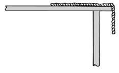
Figure 3.  Problem 9.21.

 

Let us call x the length of rope hanging over the edge of the table, and L the total length of the rope. The equation of motion is

 

 

Let us look for solution of the form

 

 

Putting this into equation of motion, we find

 

 

Initial conditions are

 

 

and

 

.

 

From these we find that

 

 

We thus conclude that

 

 

When x = L, the left end of the rope reaches the edge of the table, and the corresponding time is

 

 

To verify our calculations, let's make sure that energy is conserved.  Assume the rope has a total mass M.  We choose our coordinate system such that the vertical position coordinate on the surface of the table is 0; we also choose the surface of the table to be the plane in which the gravitational potential energy is equal to 0.  To determine the change in the potential energy of the of the rope, we examine the change in the vertical position of its center of mass:

 

 

and

 

 

The change in the potential energy is thus equal to

 

 

Note: since the rope does not stretch, there is no change in the potential energy associated with the internal forces.  To determine the change in the kinetic energy of the system, we need to determine the change in the velocity of the center of mass.  The system is initially at rest, and the initial velocity of the center of mass is thus 0 (and so is its kinetic energy).  The velocity of the system at the time the left end of the rope reaches the edge of the table can be found from the equations of motion:

 

 

When the rope reaches the edge of the table, the velocity of the center of mass is thus equal to

 

 

This equation can be rewritten as

 

 

The change in the kinetic energy of the system is thus equal to

 

 

 

 

      Elastic and Inelastic Collisions

      When two particles interact, the outcome of the interaction will be governed by the force law that describes the interaction.  Consider an interaction force F_int that acts on a particle.  The result of the interaction will be a change in the momentum of the particle since

 

 

If the interaction occurs over a short period of time, we expect to a change in the linear momentum of the particle:

 

 

This relation shows us that if we know the force we can predict the change in the linear momentum, or if we measure the change in the linear momentum we can extract information about the force.  We note that the change in the linear momentum provides us with information about the time integral of the force, not the force.  Due to the importance of the time integral, it has received its own name, and is called the impulse P:

 

 

If we consider the effect of the interaction force on both particles we conclude that the change in the linear momentum is 0:

 

 

This of course should be no surprise since when we consider both particles, the interaction force becomes an internal force and in the absence of external forces, linear momentum will be conserved.

      The conservation of linear momentum is an important conservation law that restricts the possible outcomes of a collision.  No matter what the nature of the collision is, if the initial linear momentum is non-zero, the final linear momentum will also be non-zero, and the system can not be brought to rest as a result of the collision.  If the system is at rest after the collision, its linear momentum is zero, and the initial linear momentum must therefore also be equal to zero.  Note that a zero linear momentum does not imply that all components of the system will be at rest; it only requires that the two object have linear momenta that are equal in magnitude but directed in opposite directions.

      The most convenient way to look at the collisions is in the center-of-mass frame.  In the center-of-mass frame, the total linear momentum is equal to zero, and the objects will always travel in a co-linear fashion.  This illustrated in Figure 4.

 

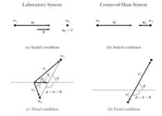
Figure 4.  Two-dimensional collisions in the laboratory frame (left) and the center-of-mass frame (right).

 

We frequently divide collisions into two distinct groups:

 

·      Elastic collisions: collisions in which the total kinetic energy of the system is conserved.  The kinetic energy of the objects will change as a result of the interaction, but the total kinetic energy will remain constant.  The kinetic energy of one of the objects in general is a function of the masses of the two objects and the scattering angle.

 

·      Inelastic collisions: collisions in which the total kinetic energy of the system is not conserved.  A totally inelastic collision is a collision in which the two objects after the collision stick together.  The loss in kinetic energy is usually expressed in terms of the Q value, where Q = K_f - K_i:

o      Q < 0: endoergic collision (kinetic energy is lost)

o      Q > 0: exoergic collision (kinetic energy is gained)

o      Q = 0: elastic collision (kinetic energy is conserved).

In most inelastic collisions, a fraction of the initial kinetic energy is transformed into internal energy (for example in the form of heat, deformation, etc.).

Another parameter that is frequently used to quantify the inelasticity of an inelastic collision is the coefficient of restitution e:

 

 

where u are the velocities after the collision and v are the velocities before the collision.  For a perfect elastic collision e = 1 and for a totally inelastic collision e = 0.

 

      One important issue we need to address when we focus on collisions is the issue of predictability.  Let's consider what we know and what we need to know; we will assume that we looking at a collision in the center-of-mass frame.  Let's define the x axis to be the axis parallel to the direction of motion of the incident objects, and let's assume that the masses of the objects do not change.  The unknown parameters are the velocities of the object; for the n-dimensional case, there will be 2n unknown.  What do we know?

 

·      Conservation of linear momentum: this conservation law provides us with n equations with 2n unknown.

 

·      Conservation of energy: if the collision is elastic, this conservation law will provide us with 1 equation with 2n unknown.

 

For elastic collisions we thus have n+1 equations with 2n unknown.  We immediately see that only for n = 1 the final state is uniquely defined.  For inelastic collisions we have n equations with 2n unknown and we conclude that event for n = 1 the final state is undefined.  When the final state is undefined we need to know something about some of the final-state parameters to fix the others.

      There are many applications of our collision theory.  Consider one technique that can be used to study the composition of a target material.   We use a beam of particles of known mass m₁ and kinetic energy T_initial to bombard the target material and measure the energy of the elastically scattered projectiles at 90°.  The measured kinetic energy depends on the mass of the target nucleus and is given by

 

 

By measuring the final kinetic energy we can thus determine the target mass.  Note: we need to make sure that the object we detect at 90° is the projectile.  An example of an application of this is shown in Figure 5.

 

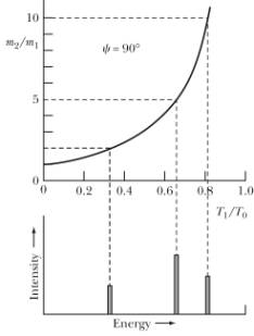
Figure 5.  Energy spectrum of the scattered projectiles at 90°.

 

 

 

      Scattering Cross Section

      We have learned a lot of properties of atoms and nuclei using elastic scattering of projectiles to probe the properties of the target elements.  A schematic of the scattering process is shown in Figure 6.  In this Figure, the incident particle is deflected (repelled) by the target particle.  This situation will arise when we consider the scattering of positively charged nuclei.

 

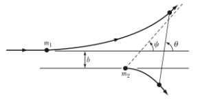
Figure 6.  Scattering of projectile nuclei from target nuclei.

 

The parameter b is called the impact parameter.  The impact parameter is related to the angular momentum of the projectile with respect to the target nucleus.

      When we study the scattering process we in general measure the intensity of the scattered particles as function of the scattering angle.  The intensity distribution is expressed in terms of the differential cross section, which is defined as

 

 

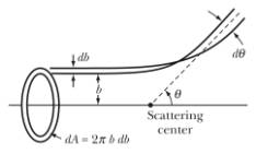
Figure 7.  Correlation between impact parameter and scattering angle.

 

There is a one-to-one correlation between the impact parameter b and the scattering angle q (see Figure 7).  The one-to-one correlation is a direct effect of the conservation of angular momentum.  Assuming that the number of incident particles is conserved, the flux of incident particles with an impact parameter between b and b + db is equal to

 

 

must be the same as the number of particles scattered in the cone that is specified by the angle q and width dq.  The area of this cone is equal to

 

 

The number of particles scattered into this cone will be

 

 

The minus sign is a result of the fact that if db > 0, dq < 0.  We thus conclude that

 

 

or

 

 

The scattering angle q is related to the impact parameter b and this relation can be obtained using the orbital motion we have discussed in this and in the previous Chapter:

 

 

The relation between the scattering angle q and the impact parameter b depends on the potential U.  For the important case of nuclear scattering, the potential varies as k/r.  For this potential we can carry out the integration and determine the following correlation between the scattering angle and the impact parameter:

 

 

where

 

 

We can use this relation to calculate db/dq and get the following differential cross section:

 

 

We conclude that the intensity of scattered projectile nuclei will decrease when the scattering angle increases.  If the energy of projectile nuclei is low enough, the measured angular distribution will agree with the so-called Rutherford distribution over the entire angular range, as was first shown by Geiger and Marsden in 1913 (see Figure 8 left).

      Each trajectory of the projectile can be characterized by distance of closest approach and there is a one-to-one correspondence between the scattering angle and this distance of closest approach.  The smallest distance of closest approach occurs when the projectile is scattered backwards (q = 180°).  The distance of closest approach decreases with increasing incident energy and the Rutherford formula indicates that the intensity should decrease as 1/T².  This was indeed observed, up to a maximum incident energy, beyond which the intensity dropped of much more rapidly than predicted by the Rutherford formula (see Figure 8 right).  At this point, the nuclei approach each other so close that the strong attractive nuclear force starts to play a role, and the scattering is no longer elastic (the projectile nuclei may for example merge with the target nuclei).

 

              

 

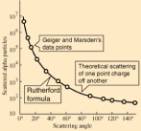
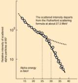
Figure 8.  Measurement of the scattering of alpha particles from target nuclei.  Figures taken from http://hyperphysics.phy-astr.gsu.edu/hbase/nuclear/rutsca2.html.