Using a Motion
Sensor
January 16, 21, & 23,
2002
Alice Tran
Lia Field
Abstract:
Motion is observable through many different facets. One facet is a motion
sensor, in which the one-dimensional motion of an object can effectively be
measured.
Theory:
Depending upon the variables of an experiment, different results occur under
different conditions. Using the motion sensor, and viewing the data through
a graph, one can view the motion of an object. The motion sensor uses pulses
that reflect from an object back to the motion sensor, and determines the
distance by the relative time difference between the emission of a pulse,
and it’s reflection. With analysis, the data will show the starting
point, displacement, velocity, and acceleration of an object during an experiment.
Graphs are very important in the analysis of the experiment, as well as the
reproduction of the motion.
Experimental:
1. The first task of the experiment was to set up the equipment. A support
rod was secured to a base, and the motion sensor was placed on the rod at
varying lengths depending upon the distance of the object. (If the object
were close by, then the motion sensor would be placed only a few inches from
the table, however, if it were a farther distance, the motion sensor should
be place at the very top of the rod, to avoid interference from the table
or other surrounding objects. And if we predicted the object to extremely
far away, then we placed the base and rod on a chair, and the motion sensor
on the top of the rod to measure this far away distance. If after a certain
point there was interference from the floor, then we concluded that we could
not measure any further, since we limited by our environment.) In addition,
the motion sensor can be turned on by pressing REC in the control window,
and it will automatically turn off after ten seconds. .
2. The second task of the experiment was to calibrate the motion sensor (which
was a Pasco sonic motion sensor). This task was accomplished by taking a ruler
and measuring the distance perpendicular to the front of the motion sensor.
After measuring a certain distance, for example .5 meters (m), we placed a
flat object at the .5 m mark, and turned on the motion sensor. If the motion
sensor also measured .5 m, then we knew it was calibrated. Of course we repeated
this several times at different lengths to reaffirm that the motion sensor
was calibrated. Once the relative accuracy of the motion sensor was known,
we tried to determine the minimum and maximum ranges of the motion sensor
at different frequencies (120, 60, and 5 hertz).
3. In addition, we tried to reproduce the motion of and object in a given
graph. After first analyzing the graph, and determining approximately where
the object started, we tried moving the object back at a similar velocity
as the graph, and then stopping at the moment the graph plateaued. After several
tries, the given graph was somewhat (although not perfectly) reproducible.
4. From the data, we were able to draw some conclusion about the motion sensor,
the different results obtained from different variables within the experiment
(such as runs at different frequencies), the effects of velocity, and acceleration
on the data.
Data Analysis:
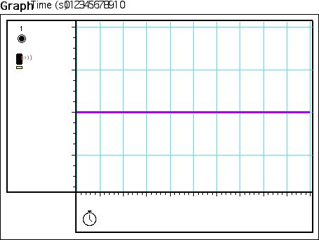
1. Data receive from the sensor could be observed through either looking at
a time/position graph, or the digital meter. For the initial testing of the
Motions Sensor (P00), the minimum reading possible was .4m (figure 1). This
was determined after several tests of various measurements lower than .4m.
The results of these tests would be much higher that what it should be (i.e.
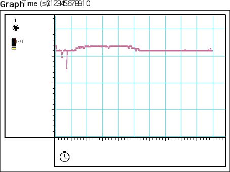
at .2 m, the senor would read .41m). The maximum was determined by seeing
how far the sensor could read a distance before it was limited by the environment,
or it started producing unexplainable readings. The maximum of P00 was 3.27m
(figure 2). Note: that we were limited is several ways to determine the actual
maximum range. First of all, we were limited by the environment, because even
if the motion sensor had the ability to detect ranges farther than 3.27m,
we could not measure it because, 3.27m was the boundary of the experiment
setup (a black box at the other end of the table). In addition, since the
sensor operates by sending sound in a cone, there is a slight discrepancy
about the maximum range. The computer is technically only 3.14maway from the
black box. However, since the motion sensor emits sound in a cone shape, the
distance measure could have been the hypotenuse distance. This hypothesis
is supported by the fact that according to Pythagorean’s theorem (a2+b2=c2),
the hypotenuse distance would be 3.21m, which is close to the 3.27 meter indicated
by the computer (diagram 1).
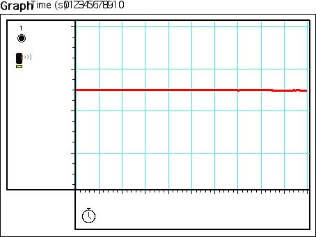
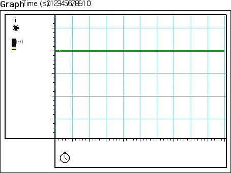
Both figures 3, and 4 show that motion sensor was calibrated, because at the
measure of .5m, the sensor read .5m (figure 3), and at the measure of 1m,
the sensor read 1m (figure 4).
Errors that might have occurred during experiment P00, (other that the measurement
of the hypotenuse), included limitations of the experiment’s environment.
These limitations include surrounding objects such as the computer, the back
box, or other things like chairs, etc. A frequent limitation was the table.
Since the sensor emitted sound as a cone, the cone often hit the table, and
reflected back, before it hit the intended object. This problem could often
be solved by raising the sensor higher, however the rod was only so tall,
thus after a certain distance the sensor would eventually be hitting the table.
2. The experiments P00a, b, and c tested for the minimum and maximum ranges
at different frequencies. P00a at 120 hertz, P00b at 60 hertz, and P00c at
5 Hertz.
|
Frequency (Hz)
|
Minimum Distance
(m)
|
Maximum Distance
(m)
|
|
120
|
.4
|
.6
|
|
60
|
.4
|
.85
|
|
5
|
.4
|
4.25*
|
* The true maximum of the sensor at 5 hertz could not be determine due to
the limitations of the environment. Interference from the table, caused the
readings to plateau. When we tried to adjust for this interference, by placing
the rod and senor on a chair, (creating more distance between the senor and the
floor) the sensor again plateaued but at a higher reading (4.25m). These tests
shows that the when the distance between the sensor and wither the table or the
floor increase, then the plateau increases. Thus the maximum measure possible
is whatever the environment permits. In this case the maximum is therefore
4.25m.
** Note, that P00a did not work due to possible equipment
defect. (Actual reason never determined, but after using a new motion sensor,
results turned out normally.)
Due to the fact that that the motion
sensors can’t distinguish between the burst it sends out, if the object is
to far away, than a reflection of burst one, may be read as a reflection of
burst 2, thus the object seems closer that it is in reality. Notice the spikes
in most figures 5-13 (excluding calibration graphs). Thus the maximum distance
a motion sensor can read is the distance at the first spike in the graph. It
might have read an object further, away, but we can accurately determine if did
because of the delay in reflection. Thus we determine that the 1st
spike should be the indicator of the maximum distance.
In P00a, we
determined the minimum by slowly moving an object farther away from the motion
sensor, and analyzing the date output. We noticed that at points before .4m,
the output were high, and consistent, then at .4m, it starting increasing.
After several tests with the same results, we concluded that the minimum for
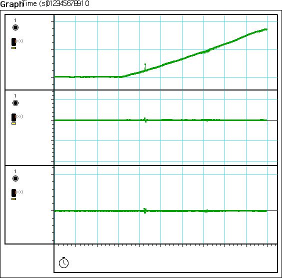
120hz was .4m (figure 5). The same method was use for finding the maximum. By
moving an object slowly farther from the motion sensor, we looked at the data
and observed any aberrations. We noticed that consistently, the slope of the
graph increased after .4m, and sharply dropped at .6m (figure 6), even if the
movement was a constant increase in distance. After several runs with the same
results, we concluded that the maximum distance was .6m at 120hz. Figure 7
shows that the motion sensor in P00a was calibrated when the measurement was
.6m, and the result was .61m (the difference could have been cause by human
error).
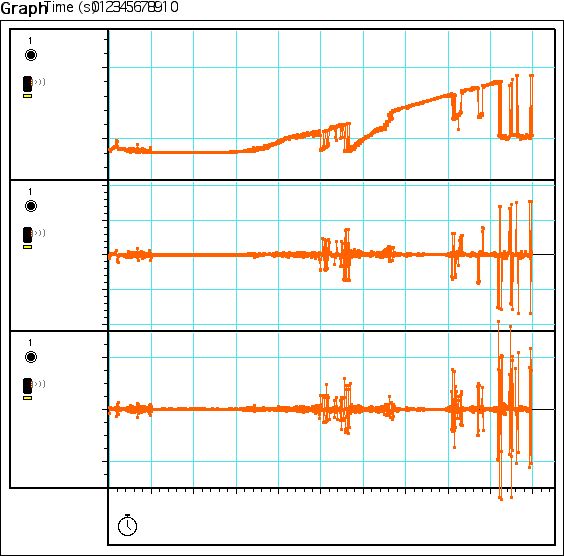 Figure 5
 Figure
6
Figure
6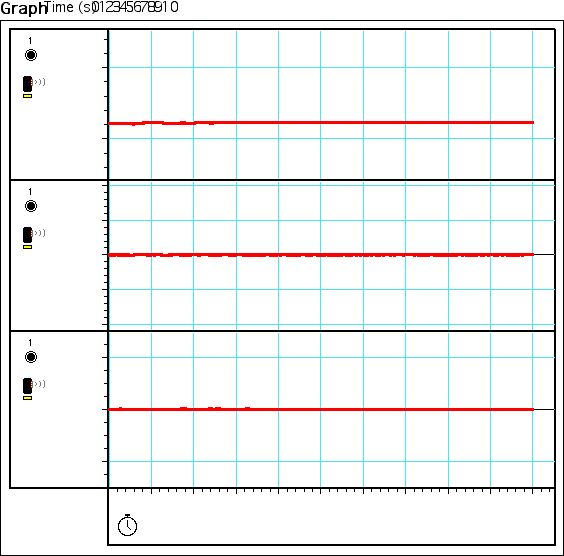 Figure
7
Figure
7We used a similar procedure in P00b as in P00a, and found that the minimum
was .4m (figure8) and the maximum was .85m (figure9), calibration at .6m equaled
.6m (figure 10) at 60hz.
 Figure
8
Figure
8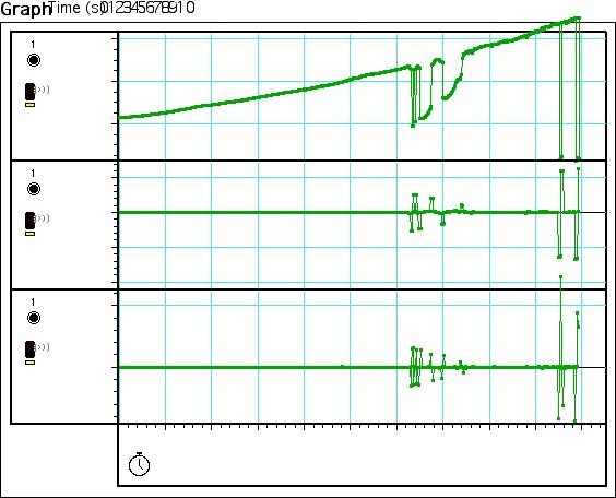 Figure
9
Figure
9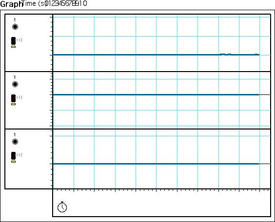 Figure
10
Figure
10In experiment P00c, we also used a similar procedure to P00a and P00b. In
determining the minimum we discovered that a points before .4m the results would
increase to about .61, and then sharply decrease to .4m when at the measurement
.4m. Thus we determined that this was the minimum point of the motion sensor at
5hz (figure 11). Starting at the minimum (.4m) we increased the distance, to
determine the maximum distance. However we discovered that after a certain
point the graph would plateau. We determined that this resulted in the
interference from the table. So we attempted to compensate by raising the
motion senor the maximum point on the rod, and then later by putting it on a
chair (thus increasing the distance between the floor and the motion sensor) to
determine the maximum distance. However even after these adjustments, we could
only measure up to 4.25m (figure 12). This point was the maximum plateau.
Although the sensor could have detected a larger distance, we were inhibited by
the environment, thus to the best of our knowledge, the maximum at 5hz is 4.25m.
The calibration for P00c is seen in figure 13, when a measurement of .5m
resulted in an output of .5m.
 Figure
11
Figure
11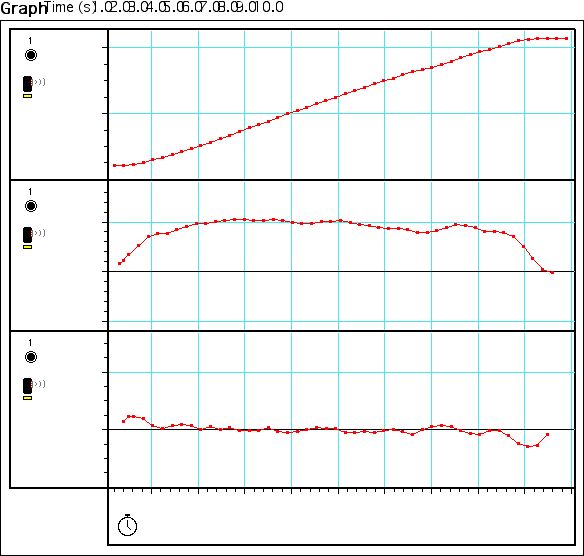 Figure
12
Figure
12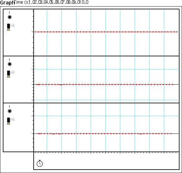 Figure
13
Figure
13Errors that might have occurred during P00a, b, and c, included the
limitations of the experiment’s environment. These limitations included
surrounding objects. The most common hindrance was the table. Since the sensor
emitted sound as a cone, the cone often hit the table, and reflected back,
before it hit the intended object. This problem could often be solved by
raising the sensor higher, however the rod was only so tall, thus after a
certain distance the sensor would eventually be hitting the table. In an
attempt to determine a farther distance, we tried putting the base/rod on the
chair, creating a taller effect, however eventually the cone hit the floor, and
we had run out of solutions. Thus even if the motion sensor could read a longer
distance, we could not prove this distance, due to the limitation of our
environment. Conversely, if the sensor was too high, and the object too small,
the cone could have missed the object completely (although we usually accounted
for this, and thus had no data with this type of error).
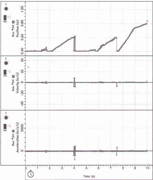
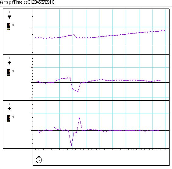
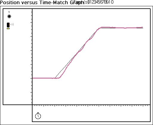
3. In
experiment P001 attempted to duplicate and experiment by tracing over the
initial experiment’s graph. First we analyze the graph, and determined
the starting point to be .4m. It is plateau at .4m, which indicated that the
object is stationary. Then the distance increased at a certain velocity, and
again plateaus at around 2.7m. With this information and the use of trail and
error, we were able to reproduce the experiment with close degree of accuracy.
In figure 14, the graph appears to quite similar to the original graph, with a
chi-square of .085342. However we were able to improve the chi-square in figure
15 to .060071. The difference between the two graphs is very interesting
because although figure 14 looks better than figure 15, figure 15 has more
accurate points, and thus is a better reproduction of the experiment. Thus
proving that looks can be deceiving, and analysis of a graph can’t a
superficial glance at a graph, but also a more in depth look at the data.
 Figure
14
Figure
14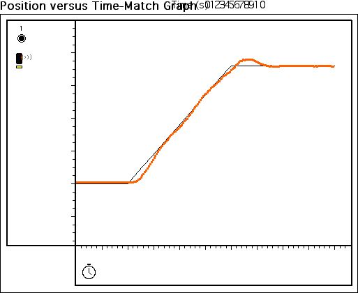 Figure
15
Figure
15
Conclusions:
This experiment showed that at different frequencies, the range of measurement
different. Hence the lower the frequency the longer the distance that could
be measure, because the difference between burst was longer. Also, the motion
sensor experiment has showed that one can’t take the data result at
face value. One must not only analyze the graphs, but also determine what
they mean. A graph may seem to show the distance of an object, however in
reality, a slight aberration that could easily be over looked, may have important
meaning. Although a graph may continue to increase as the object increases
after a spike, this does not mean that it is a correct distance. A spike is
an indication that the object is out of range, that the first burst is being
reflected back after the second had been emitted, creating faulty data if
interpreted wrongly. Thus once a spike occurs, we determined that at this
point is the maximum distance the motions sensor can measure. In addition,
when the graphs each experiment we look into closely, we noticed that there
were several small aberrations, even though the digital meter may have output
a consistent number. This shows that the graph may seem accurate; there may
be slight discrepancies. However for the most part, the motion sensor measures
distance within acceptable parameters.
Also, after observing the velocity and acceleration graph while moving an
object, I noticed that velocity was positive, when the object moved further
away, and was negative when there was a decrease in distance. In addition,
the acceleration was positive when the velocity increase, but was negative
when it decreased.
Finally, errors occurred usually due to physical limitations, such as surround
object interfering with reading the moving object, and the limited range caused
by lack of height. Other errors included measuring the horizontal distance,
when the sensor when the hypotenuse distance, and simple human error. However
for the most part, this lab went smoothly as predicted.
Remarks:
This experiment was very useful in showing that error often occurs, and that
one must closely analyze the data before coming to a conclusion. And although
we never were able to determine why the experiment didn’t work the second
day of class, I was thankful, that the experiment began to go well the follow
lab.