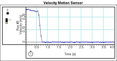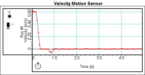
Figure 1. Velocity graph with a motion sensor
for Run 1
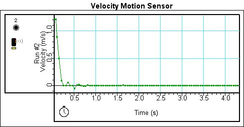
Figure 2. Velocity graph with motion sensor
for Run 2.
Abstract:
In this lab we used a photo gate in combination with a motion sensor to study instantaneous velocity, average velocity and the difference between the two types of velocity. Video analysis was also used in this lab to aid in the analysis.
Theory:
The parameters position, velocity and acceleration are most commonly used to describe one dimension motion. Velocity is the change of position over the change of time. Instantaneous velocity is the velocity of an object at a certain point in time whereas average velocity is the ratio of the total distance an object travels over a set time period and the set time period it takes the object to travel that certain distance. Velocity can be constant, positive, or negative. A constant velocity is a velocity with no acceleration. Velocity is positive when the object is moving forward with either positive or negative acceleration and velocity is negative when the object is moving backward with either positive or negative acceleration. Two different devices, the motion sensor and the photo gate, can be used to measure velocity. A motion sensor measures the position of objects at fixed time intervals and computes the velocity from the differences in the readings. The photo gate works the opposite way, measuring the time of an object when it reaches fixed distance intervals and calculates the velocity by the difference between the readings. Besides being measured by a motion sensor and photo gate, velocity can also be measured by taking the motion of an object and completing a video analysis.
Experiment:
Data Analysis:
Figure 1. Velocity graph with a motion sensor
for Run 1
Figure 2. Velocity graph with motion sensor
for Run 2.
Figure 3. Velocity graph with motion sensor for Run 3.
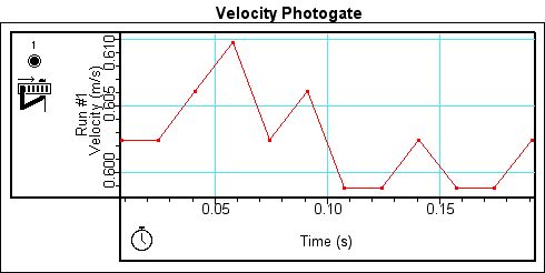
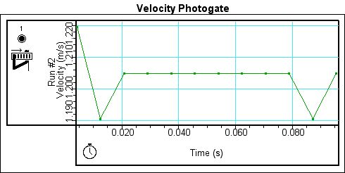
However, when velocity is measured by the photogate, the graphs do not show the same trend. Instead, three different graphs are produced with no similar characteristics. The differences in the graphs could be due to the way that the photogate measures velocity. Figure 5 shows the graph for the largest initial velocity. If one notes in the graph there is a constant velocity for about .06 sec. It is possible that at such as high velocity the cart whizzed right through the photogate, barely slowing down, explain the constant velocity on the graph. Figure 4 is the velocity graph of the medium initial velocity. The graph of the velocity shows a downward trend regardless of the spikes that appear in the graph. Figure 6, which is the velocity graph of the lowest initial velocity, demonstrates a curve which is similar to those seen when measuring velocity with a motion sensor.
Figure 4. Velocity graph with photogate for Run 1.
Figure 5. Velocity graph with photogate for Run 2.
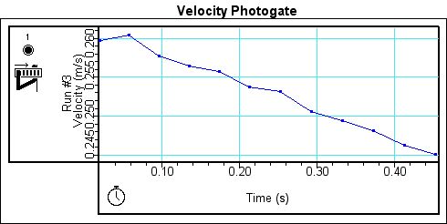
Figure 6. Velocity graph with photogate for Run 3.
Because both the motion sensor and the photogate are measuring the same motion, it would be expected that the data from both the motion sensor and photogate would correspond with each other. Figures 7 and 8 are the velocity-velocity graphs for runs 1 and 3. The velocity-velocity graph for each run plots the velocity measured by the motion sensor against the velocity measured by the photogate.
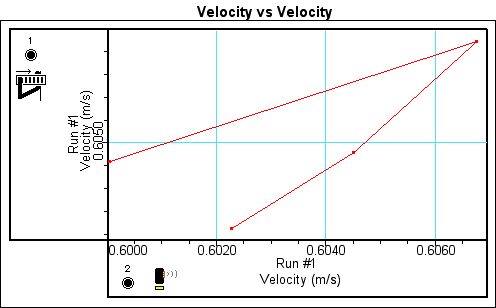
Figure 7. Velocity vs. Velocity for Run 1
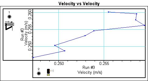
Figure 8. Velocity vs. Velocity for Run 2
While the majority of the points on each velocity vs. velocity graph do not correspond with each other exactly, many points are only slightly off, proving that the motion sensor and photogate measure the same velocity.
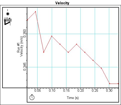
Figure 9. Run 1's Velocity Graph, Smallest Initial Velocity
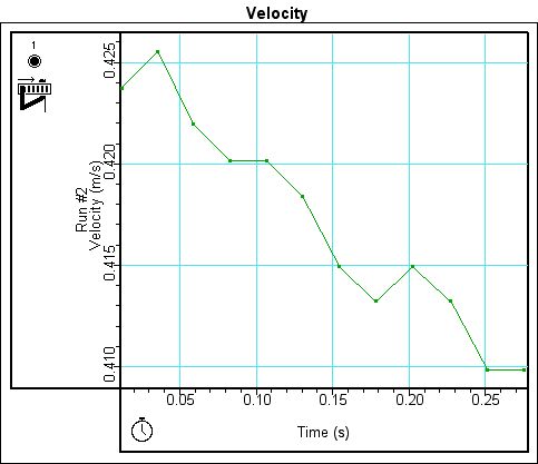
Figure 10. Run 2's Velocity Graph
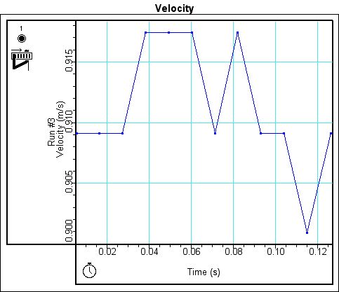
Figure 11. Run 3's Velocity Graph, Largest Initial Velocity
|
Height 21 cm
|
|
|
Trial #'s
|
Distance between photogates (cm)
|
|
1-3
|
40
|
|
4-6
|
30
|
|
7-9
|
20
|
|
10-12
|
10
|
Table 1. Distance data for Run 1
|
Height 26 cm
|
|
|
Trial #'s
|
Distance between photogates (cm)
|
|
1-3
|
40
|
|
4-6
|
30
|
|
7-9
|
20
|
|
10-12
|
10
|
Table 2. Distance data for Run 2
|
Height 30 cm
|
|
|
Trial #'s
|
Distance between photogates (cm)
|
|
1-3
|
40
|
|
4-6
|
30
|
|
7-9
|
20
|
|
10-12
|
10
|
Table 3. Distance data for Run 3
For each different distance between the two photogates we took three different measurements to ensure accuracy. Table 4 shows the data for each different distance as well as the margin of error for each distance for run 1 as a sample of the margin of error encountered on each run.
|
Trial #
|
Distance between photogates
(cm)
|
Average Speed (m/sec)
|
Margin of Error
|
|
1
|
40
|
.5820
|
+/-.0005
|
|
2
|
40
|
.5835
|
|
|
3
|
40
|
.5830
|
|
|
4
|
30
|
.575
|
+/-.0023
|
|
5
|
30
|
.574
|
|
|
6
|
30
|
.568
|
|
|
7
|
20
|
.5510
|
+/-.00083
|
|
8
|
20
|
.54950
|
|
|
9
|
20
|
.54850
|
|
|
10
|
10
|
.5105
|
+/-.0003
|
|
11
|
10
|
.5080
|
|
|
12
|
10
|
.5080
|
Table 4. Distance and Margin of Error data for Run 1
Figure 12 displays the graphs for runs 1, 2 and 3 for the average speed of experiment P03. If one was using the graph of the average speed in trying to determine the instantaneous speed, the measurement that would most accurately reflect the instantaneous speed on the graph would be the data points to the farthest right of the graph, or the data points taken with the least distance between the photogates. The graph of the instantaneous velocity for runs 1, 2 and 3 is displayed by Figure 13 for comparison to the average speed graphs of Figure 12.
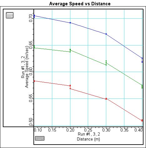
Figure 12. Average Speed Graphs for Runs 1, 2 and 3
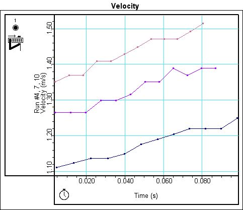
Figure 13. Velocity Graphs Corresponding to Heights Used in P03
Conclusion:
Through our experimentation with velocity, using
two different ways of collecting data, both the motion sensor and the photogate,
we were able to explore average, instantaneous and constant velocity. With
our first experiment comparing the results of the motion sensor and the photogate
we discovered that even though each instrument had separate ways of collecting
data, both were consistent in the way they collected and displayed data. While
the data from the motion sensor and the photogate did not correlate exactly,
the data was not so far away each other that we determined that both the photogate
and motion sensor were accurately able to detect velocity. Next using just
the photogate, we discovered that the velocity graph of an object that at
first appeared constant upon closer inspection was not, enforcing the idea
that constant velocity is when the velocity of an object remains constant,
meaning the velocity is neither increasing or decreasing. Measurement of velocity
besides taken by the motion sensor or photogate was also explored when we
used the stills from a video clip to determine the motion of a lunar module
and a space shuttle. Since we knew the time increment between each still,
by determining the height of the object in each still, it was easy to find
the velocity graph. Finally in experiment P03 the relationship between instantaneous
velocity and average velocity was explored. It was determined that when plugging
in an x value on the average velocity graph that the corresponding y value
does not produce the accurate instantaneous velocity for that value of x.
Instead the y value of the average velocity graph is more like a rough estimate
for the instantaneous velocity. However, the more data points that make up
the average velocity graph, the closer the y value is to being the correct
instantaneous value. Average velocity is normally calculated by taking the
distance over the time taken to travel that distance. No such simple formula
exists for finding instantaneous velocity, but devices such as a motion sensor
or photogate can measure instantaneous velocity.
Remarks:
Learning about the differences between average
and instantaneous velocity was fun. However, the experiments could have been
accomplished a lot less painstakingly and in less time by my partner and I
if we had been aware of the photogate cord interfering with the cart earlier.