NOTE
This manual describes the laboratory experiment used during the 1996 - 1997 academic year. Significant changes have been made since then, and the manual used during the current academic year is in NOT available yet on the WEB. Hardcopies can be purchased at the bookstore.
To calculate an absolute voltage measurement by mechanical means and illustrate the concepts of the electric field by means of experimental demonstration.
The prelab homework must be done at home and handed to the lab TA before you start the lab. Read the instructions for this lab.
1) What is the expression for the stored energy in a capacitor in terms of capacitance and voltage?
2) Derive the expression for the buoyant force ![]() given in the write up.
given in the write up.
3) What are students supposed to learn by doing the lab?
A force (given by Coulomb's Law) is exerted on a particular electric charge by every other charge. The total electrical force acting on such a charge is the sum of all these forces. If a small charge were introduced to "test" it, the force on this test charge would be found to vary as it was moved around.
Considerations such as these give rise to the concept of a field. The force per unit test charge is a function of position in space that is independent of the test charge and characteristic of the spatial distribution of charge in the region. At any location the electric field (due to an array of charges, for example) is defined as the electric force per unit charge (i.e.. the force that would be exerted on a unit positive charge) at that point. The electric field can be thought of as the capacity for producing an electric force on a charge. Conceptually, the electric field is well defined at any place even though there may not actually be any test charge there to experience it.
If a test charge is moved around in an electric field, work will be done on it by the electric force. The static electrical force of Coulomb's law is a conservative force. That is, the work done moving between two points is independent of the path taken. This suggests another useful concept, electric potential. The potential difference between two points is the work per unit charge that would be done by the electric field in moving a test charge between them.
Such experience should help the student gain a concrete grasp of these abstract concepts and facilitate understanding of capacitance and the connection between force, distance and energy in the context of electrical phenomena.
In the first part of this experiment, you will relate an electrical potential to mechanical quantities using an indirect method to make an absolute voltage measurement. This method, through clever design, avoids the worst of the systematic errors from which a direct Coulomb's Law experiment suffers and yields more precise results. The ability to design experiments which yield results with small systematic errors is what distinguishes the best experimental scientists. In the second part, you will investigate static electric fields and map out their potentials.
An absolute measurement of electrical potential difference (V-voltage) by mechanical means is a way to learn about electrical quantities and relate them directly to mechanical ones that are already understood. Along the way other familiar phenomena will be verified.
The study of electricity and magnetism normally begins after a thorough introductory study of mechanics. The first important electrical relationship encountered is Coulomb's law, which says that the force acting between two point charges is proportional to their magnitudes and inversely proportional to the square of the distance between them. Once the constant of proportionality has been chosen the unit of charge has in principle been defined for that system of units(i.e. m.k.s.). Then, in order to measure charge one would simply set up two identical point charges a known distance apart, measure the force between them and then use Coulomb's law to get the magnitude of the charges.
But making direct, accurate Coulomb's law measurements is not readily feasible. The required point charges are not available, and the distribution of charges on conducting spheres (such as one might try to use in practice) is not uniform. The distribution of charge depends in a complicated way on the position of all local objects, conducting or non-conducting, charged or not charged.
Fortunately, a practical way exists to determine an electrical quantity in terms of force, by making an "absolute" measurement, using a method based on capacitance.
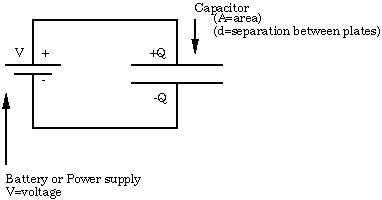
Figure 7.1
Since the charge on an electrical conductor distributes itself so as to form an equipotential, there is a certain value of electrical potential associated with each conductor. And, because electrostatic fields superimpose, these potentials will be linearly related to the charges on the conductors. The concept of capacitance describes the coefficients of these relationships, which are determined only by the geometry.
In a system of two-conductors which carry opposite charges of magnitude Q, this relationship is simply,
Q=CV (7.1)
where V is the voltage (potential difference) between them, and the coefficient C is their mutual capacitance. A simple example is the parallel plate capacitor, which has a capacitance in air (neglecting edge effects) of,
![]() (7.2)
(7.2)
![]() 0 (= 8.854
0 (= 8.854 ![]() 10-12 Coulombs2//Newton
Meters2) is the dielectric constant of free space.
10-12 Coulombs2//Newton
Meters2) is the dielectric constant of free space.
In a capacitor one plate has positive charges on it and the other has negative. These charges attract so, as expected, the plates of such a capacitor exert attractive forces on each other. This force can be obtained, given the charge distribution on the charged capacitor, by integration.
However, it is also possible to approach this problem from the point of view of the principle of virtual work. The stored electrical energy of such a system is,
![]() (7.3)
(7.3)
Since this energy changes as the geometry (and hence C) changes, it must require work to move the plates of a capacitor. It is the force Fe that the plates of the capacitor exert on each other that does this work. Thus, if C depends on a single dimension z the magnitude of the force between the electrodes (i.e.. the rate at which work is done per unit displacement) in the direction of that variable, assuming V is constant, is,
![]() (7.4)
(7.4)
In the parallel-plate case this is,
![]() =
= ![]() (7.5)
(7.5)
Note the quadratic dependence of the force on the voltage and that the constant of proportionality, apart from an electrical physical constant, is purely geometric. Therefore, if the force between the plates can be measured, the potential difference V can be calculated immediately. From the above example the voltage is calculated from,
![]() (7.6)
(7.6)
This is the principle on which this experiment is based. However, for practical reasons the capacitor will be two concentric cylinders rather than parallel plates. The axis of the cylinders will be in the same direction as the force (+z). Of course, the capacitance between the two cylinders will be different from the capacitance of the parallel plate, example shown above, but capacitance depends only on the dimensions. This is discussed below.
The apparatus shown in Figure 7.2 is designed for measuring the axial force in the vertical z direction between two concentric aluminum circular cylinders. The potential difference is determined across these two cylinders where up to 3,000Volts is applied. The outer cylinder of the capacitor is fixed in the semicircular ends of two Lucite plates. The inner cylinder, which must be quite uniform and light in weight, is made from a cleaned beverage can.
This inner cylinder moves vertically supported by a thin shaft constrained by two bearings. These bearings must run freely; so they must be kept clean. If a bearing begins to rub or grab it can be washed out with alcohol and then lubricated with a small single drop of spindle oil. The lower end of the shaft is supported by a hollow float partially submerged in water. Distilled water with a few drops of Eastman Kodak Photo-Flo 200 wetting agent will reduce surface tension. The fully submerged main body of the float, a ping-pong ball (of unknown compressibility), provides most of the buoyancy required to support the shaft and its load. The submerged portion of the glass tube connecting the ball to the shaft supplies the rest.
The total vertical force on the movable part of the experiment is,
![]() (7.7)
(7.7)
![]() is the electrical force
between the cylindrical capacitors;
is the electrical force
between the cylindrical capacitors; ![]() is the upward buoyancy force of the ping-pong ball, and
is the upward buoyancy force of the ping-pong ball, and ![]() is the downward force of gravity. The idea
is for
is the downward force of gravity. The idea
is for ![]() and
and ![]() to almost cancel each other so that
to almost cancel each other so that
![]() dominates.
dominates.
The (vertical) equilibrium position is set by the water level in the beaker and the small weights (brass or steel nuts) in the weight pan. The weights should be used to adjust the immersion of the float so that the surface of the water is level with the center of the rod. The water level should be adjusted so that the can clears the top bearing by about a centimeter.
The system will be displaced from equilibrium by any force between the cylinders. This rather high sensitivity is easy to estimate from physical principles (see figure 7.2). The position of the system is observed through a low-power microscope directed at an optical target on the shaft.
The can is connected to ground via the bearings, the outer cylinder is connected to the potential source through a protective (high voltage) resistance of several tens of mega-ohms. Although this high voltage is exposed, the resistor prevents any significant current from flowing; it is not dangerous, although it may be uncomfortable if touched. Therefore, do not touch the can which could be at 3000V.
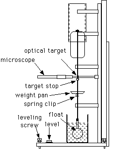
Figure 7.2
The can and cylinder overlap for a length much greater than the radial spacing between them, and the cylinder extends well beyond the upper end of the can. Under these conditions the change in capacitance produced by a small axial position shift s will, to a very good approximation, be given simply by,
![]() (7.8)
(7.8)
where ( ![]() is the outer
radius,
is the outer
radius, ![]() is the inner
radius) and,
is the inner
radius) and,
![]() =
= ![]() (7.9)
(7.9)
is the capacitance per unit length of a long cylindrical capacitor
having electrodes with the same geometry as the apparatus;
![]() and
and
![]() are the radii of the
cylinder and can, respectfully. This is because the electrical
field distribution in most of the overlap region is essentially
invariant axially; and also the end effects will be quite small
due to the favorable geometry (the cylinder extends well beyond
the can above and the can extends well beyond the cylinder below).
are the radii of the
cylinder and can, respectfully. This is because the electrical
field distribution in most of the overlap region is essentially
invariant axially; and also the end effects will be quite small
due to the favorable geometry (the cylinder extends well beyond
the can above and the can extends well beyond the cylinder below).
Think of the capacitance associated with each of the three distinct regions: the overlap region (where the electrical field is invariant axially), the upper end and the lower end. If the can moves, say upward, the overlap will lengthen and the capacitance will increase linearly with s.
The top will move upward toward the open end of the cylinder, so its part of the capacitance will get smaller, but the end of the cylinder is so far away that the change will be quite small. A similar argument can be made with regard to the lower end, since the can extends considerably below the cylinder.
Accordingly, for a potential difference of V between the electrodes, the change in energy storage with displacement may be written,
![]() =
= ![]() =
= ![]() (7.10)
(7.10)
By the principle of virtual work, the force is the derivative of dU with respect to s. Therefore,
Fe = ![]() =
= ![]() =
= ![]() (7.11)
(7.11)
is the force acting on the can due to electrical effects.
The system will float at equilibrium where all the forces due to gravity, buoyancy and electrical effects balance out. The system is constructed so that the constant force of gravity is mostly canceled out by the buoyancy of the fully submerged ping-pong ball. Thus changes in the electrical forces due to the potential of the cylinder will be balanced by the changes in buoyancy due to the changed level of the float in the water.
These changes in the buoyant forces arise from changes in the water displaced by the float, which is that due to the stem (small glass tube) since the ball is always submerged. The weight of this displaced water is,
Fb= ![]() (7.12)
(7.12)
where r is the density of water and d is the diameter of the tube. The factor in brackets accounts for the small absolute level change of the water in the vessel (D is its diameter) due to the displacement.
Since Fb is small for the thin tubing, the apparatus is very sensitive to the magnitude of the electrical force, and it can be estimated from the observed displacement of the shaft and the known geometry of the float system.
Combining the above expressions gives the applied voltage,
V2 = ![]() (7.13)
(7.13)
in terms of the displacement and the parameters of the system. (Note that r=1000 Kg /m3 in m.k.s. units.) The right hand of the equation depends only on mechanical quantities.
CAUTION: Do NOT touch the can. Although the available power is too small to be dangerous, potentials of several thousand volts are involved here so touching the cylinder may be uncomfortable. Also, if it gets dirty the experiment may fail.
1) Check to see if the water level is about halfway up the glass stem of the float; if not, add or remove weights to make it so. Check to see that the can clears the upper bearing properly (about cm). If necessary add or remove water.
For accurate and reproducible measurements the shaft must be able to freely assume its proper position. Even when the bearings are well aligned and the shaft is essentially vertical, bearing friction will interfere with the necessary free movement. This can be overcome by setting the system spinning by gentle use of thumb and forefinger on the shaft. You may find it useful to steady your hand by resting it lightly on the bearing support while doing this. Make sure your hands are clean when spinning the shaft, wash them if necessary.
2) Fiddle with the apparatus to become familiar with it. Try spinning the shaft gently using (clean and dry) thumb and forefinger. Once started, spinning should persist for five or ten seconds and should gradually die out rather than come to a sudden stop. Check to see if your apparatus behaves this way; if not the bearings need to be cleaned and you should get your TA's help.
Important: Every time you make a change you must spin the shaft to overcome the friction. Do this at least twice to confirm that you are obtaining an accurate reading.
3) Look through the microscope. If necessary reset the optical target to center it on the scale. Make sure the target will not move during your experiment by moving the target stop up to support the target. Spin the shaft and observe how the target settles into position. Repeat, checking for consistency.
Measure Displacement per Mass
4) With zero voltage applied to the apparatus find the displacements produced by five different masses. Suggested masses are: 0, 20, 40, 60, 80 milligrams.
The scale in the microscope is 6mm long with 0.1mm per minor division. Note that by knowing the spacing of the target marks (about 4mm), you can extend your range of measurement by sighting on one or the other. Measure the actual length of your target so you can do this.
Measure Displacement vs. Voltmeter Reading
5) Apply five different voltages as indicated by the power supply meter to the apparatus, ranging up to near 3000V. Suggested voltages are: 0, 1000, 2000, 2500, 3000Volts. Again spin the shaft at least twice after changing the voltage to make sure you are getting the consistent measurements.
Measure a Voltage Using the Theoretical Sensitivity
6) Set your power supply to some intermediate voltage(i.e. 2500 Volts) and make a note of the meter reading.
7) Switch the apparatus to ground and note the scale reading.
8) Then switch to the power supply voltage and record the reading. Subtract to get the displacement.
9) Repeat several times and average the values found.
10) Then calculate the applied voltage using the equation (7.13) and your system's geometric parameters (see drawing, and use m.k.s. units). How does this compare with the meter on the power supply?
Measure a Voltage Using the Null Method
11) Without changing the power supply find another value for the applied voltage by use of a null method. With the power supply off or disconnected, note a "zero" point on the scale.
12) Then apply the voltage from the power supply (i.e. 2500 Volts).
13) Keeping records, add masses until the zero point has been passed, then interpolate to find the mass corresponding to scale zero.
14) Switch off all POWER when you are done.
1) Plot using the data from 4) Mass vs. Displacement. A linear dependence should be found.
2) Observe the displacements from the data calculated in 5) for each and plot Displacement vs. Volts2. A linear dependence on V2 is expected as equation (7.12) indicates.
3) Convert the mass corresponding to scale zero to force (F=mg) and calculate a value for the applied voltage via equation (7.10). Here only stability of the zero point is required; the buoyancy force does not appear in the calculations. How does your result compare with the meter on the power supply.
4) Equation (7.10) converts this force to absolute Volts2. Step 2 gives the indicated Volts2 per displacement(mm). The square root of their ratio gives a calibration constant for the meter, which if the meter were accurate, would be one. How accurate is the meter? Discuss your results. What voltage measurement do you think is most reliable? Why? Is the power supply meter accurate ?
In this experiment you will investigate the electric potentials set up by electrodes which cause currents to flow in conductive sheets. You will be able to map out the equipotential contours and find the electric field lines for several configurations of electrodes.
The apparatus (see Figure 7.3) includes a board which holds a sheet of special paper with a conducting graphite surface, a battery, test electrodes and a galvanometer.
The paper is imprinted with an electrode pattern, and grid lines are drawn for reference purposes. It is mounted on the base with the spring clips contacting the silver electrodes. The battery is connected to the binding posts to apply a potential difference (voltage) between the electrodes.
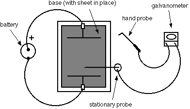
Figure 7.3. Field Mapping Apparatus
In a conductor, such as the silver electrodes, even small electric fields will cause large amounts of charge to move in such a way as to tend to cancel out the field. Thus charges will distribute themselves on the electrodes so as to make them equipotential surfaces. The field between the electrodes will be that appropriate to the resulting distribution of charges.
The graphite surface of the paper, on the other hand, has a much higher resistance than the electrodes. Small currents will tend to flow along the electric field lines (i.e. between the potential differences) set up by the charged electrodes but these will not be sufficient to significantly disturb the field pattern. By providing a source for the small current needed to drive a galvanometer, the graphite surface makes it possible for you to measure the potential differences in the electrostatic field pattern set up by the charged electrodes. The current that will flow through the galvanometer connected between two points on the paper is proportional to the potential difference between the points. Thus, by finding points between which the galvanometer measures no current, you can map out contours with the same potential.
Use the following procedure to map out the fields for the three different electrode patterns. These are:
1) two-points pattern
2) parallel-plate pattern
3) Faraday ice-pail pattern
Tabulate your measurements and results for each on one of the worksheets available at the end of the lab. Start by tracing the electrode configuration on your sheet and marking the positive electrode.
1) The galvanometer is connected to two field probes. Place the mounted probe at a reference position somewhere between the two electrodes.
2) Mark this position on your data sheet.
3) Then move the point of the hand probe over the paper to find a place giving a zero "null" reading on the meter.
4) Mark this equipotential point on the graph. In order to ensure good contact, it may sometimes be necessary to gently agitate the probe tips a bit.
5) Without moving the mounted probe, locate a whole series of null points across the paper and mark the position of each on the data sheet.
6) When you have found enough points to draw a smooth line through them, do so. This is an equipotential contour and the potential between any points on this line is zero.
7) Now move the mounted probe to a new position (not on your old contour) and map out another contour by repeating steps 1-6.
a). Map out at least four equipotential lines for the two-point and parallel-plate. In the parallel plates pattern be sure you probe beyond the ends of the plates because interesting things happen there.
b). Map out at least eight equipotential lines for the Faraday Ice-pail pattern. Make sure to do a contour quite close to one of the electrodes. Sketch as many equipotentials as is necessary to show its interesting structure. In the Faraday's ice-pail pattern start probing by putting the mounted probe near the bottom of the "pail."
8) The electric field is everywhere perpendicular to the equipotentials. Sketch in with dashed lines on your data sheets examples of how the electric field lines (lines of force) must run. Be sure to do this in the interesting parts of the pattern. Remembering that the electric field is a vector, indicate with arrows the direction associated with the electric field lines.
Note: The data sheets should be completed before you leave the lab and handed in (with answers to the questions below) with your report.
9) BE SURE TO DISCONNECT THE BATTERY WHEN YOU ARE DONE !
1) Two points pattern: In which region(s) would the electric force on a test charge be largest?
2) Parallel plates patterns: Does the electric field strength change within the region between the plates? Describe the trajectory of a positive unit charge if it were introduced midway between the plates with a velocity directed parallel to the plates.
3) Faraday's ice-pail patterns: Is the electric field inside the pail larger or smaller than that outside? Where is greatest concentration of charge on the electrodes?
4) By sketching in the field lines what is the direction of the force that would be exerted on a positive test charge?
H.W. Fullbright, American Journal Physics.(61) (10), Oct. 1993 [A Simple and Inexpensive Teaching Apparatus For Absolute Measurement of Voltage]
Data Sheet
Electric Field Mapping
Two Point Pattern
Name:________________________________________

Data Sheet
Electric Field Mapping
Parallel-Plates Pattern
Name:________________________________________

Data Sheet
Electric Field Mapping
Faraday's Ice-Pail Pattern
Name:________________________________________