Introduction.

In all branches of physical science and engineering one deals constantly with numbers which results more or less directly from experimental observations.  Experimental observations always have inaccuracies.  In using numbers that result from experimental observations, it is almost always necessary to know the extent of these inaccuracies.  If several measurements are used to compute a result, one must know how the inaccuracies of the individual observations contribute to the inaccuracy of the result.  If one is comparing a number based on a theoretical prediction with one based on experiment, it is necessary to know something about the accuracy of both of these if one is to say something intelligent about whether or not they agree.

 

Systematic Errors.

Systematic errors are errors associated with the particular instruments or techniques used to carry out the measurements.  Suppose we have a book that is 9" wide.  If we measure its width with a ruler whose first inch has previously been cut off, then the result of the measurement is most likely to be 10".  This is a systematic error.  If a thermometer immersed in boiling water at normal pressure reads 102 C, it is improperly calibrated.  If readings from this thermometer are incorporated into experimental results, a systematic error results.  A voltage meter that is not properly "zeroed" introduces a systematic error.

An important point to be clear about is that a systematic error implies that all measurements in a set of data taken with the same instrument or technique are shifted in the same direction by the same amount.  Unfortunately, there is no consistent method by which systematic errors may be treated or analyzed.  Each experiment must in general be considered individually and it is often very difficult just to identify the possible sources, let alone estimate their magnitude, of the systematic errors.  Only an experimenter whose skills have come through long experience can consistently detect systematic errors and prevent or correct them.

 

Random Errors

Random errors are produced by a large number of unpredictable and unknown variations in the experiment.  These can result from small errors in judgment on the part of the observer, such as in estimating tenths of the smallest scale division.  Other causes are unpredictable fluctuations in conditions, such as temperature, illumination, line voltage, any kind of mechanical vibration of the experimental equipment, etc.  It is found empirically that such random errors are frequently distributed according to a simple law.  This makes it possible to use statistical methods to deal with random errors.

 

Propagation of errors - Part I

If one uses various experimental observations to calculate a result, the result will be in error by an amount that depends on the errors made in the individual observations.  For example, suppose one wants to determine the area (A) of a sheet of paper by measuring its height (h) and its width (w):

                                                       (1)

Suppose that the measured height differs from the actual height by ∆h, and the measured width differs from the actual width by ∆w (see Figure 1).

 

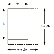
Fig.1. Propagation of errors in the measurement of area A

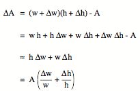
In this case the calculated area will differ from the actual area A by ∆A, and ∆A will depend on ∆h and ∆w:

     (2)

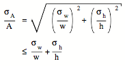
The fractional error in A, which is defined as the ratio  of the error to the true value, can be easily obtained from equation (2):

In this example, the fractional error in A depends only on the fractional errors in w and h.  However, this is not true in general.

 

Measurement Errors

If the errors in the measurements of w and h in the previous section were known, one could correct the observations and eliminate the errors.  Ordinarily we do not know the errors exactly because errors usually occur randomly.  Often the distribution of errors in a set observations is known, but the error in each individual observation is not known.

Suppose one wants to make an accurate measurement of w and h to determine the area of the rectangle in Figure 1.  If we make several different measurements of the width, we will probably get several different results.  The mean of N measurements is defined as:

                                       (4)

where wi is the result of measurement # i.  In the absence of systematic errors, the mean of the individual observations will approach w.  The deviation di for each individual measurement is defined as:

The average deviation of the N measurements is always zero, and therefore is not a good measure of the spread of the measurements around the mean.  A quantity often used to characterize the spread or dispersion of the measurements is the standard deviation.  The standard deviation is usually symbolized by s and is defined as:

The square of the standard deviation s2 is called the variance of the distribution.  A small value of s indicates a small error in the mean.  It can be shown that the error in the mean obtained from N measurements is unlikely to be greater than s/N1/2.  Thus, as we would expect, more measurements result in a more reliable mean.

 

The Gaussian Distribution

The Gaussian distribution plays a central role in error analysis since measurement errors are generally described by this distribution.  The Gaussian distribution is often referred to as the normal error function and errors distributed according to this distribution are said to be normally distributed.  The Gaussian distribution is a continuous, symmetric distribution whose density is given by:

The two parameters m and s2 are the mean and the variance of the distribution.  The function P(x) in equation (7) should be interpreted as follows: the probability that in a particular measurement the measured value lies between x and x+dx is P(x)dx.  The normalization factor in eq. (7) is chosen such that:

This relation is equivalent to stating that the probability that the result of a measurement lies between -∞ and ∞ is 1 (which is of course obvious).

The shape of the Gaussian distribution for various values of s is shown in Figure 2.  A small value of s obviously indicates that most measurements will be close to m (small fractional error).

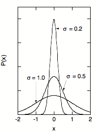
Fig.2.    The Gaussian distribution for various s.  The standard deviation determines the width of the distribution.

In many applications the measurement errors are given in terms of the full width at half maximum (FWHM).  The FWHM of a Gaussian distribution is somewhat larger than s:

            (9)

The Gaussian distribution can be used to estimate the probability that a measurement will fall within specified limits. Suppose we want to compare the result of a measurement with a theoretical prediction.  If the measurement technique has a variance s2 the probability that the result of a measurement lies between m - ns and m + ns is given by:

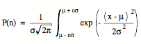    (10)

The following table shows equation (9) evaluated for several values of n.

For example, the oscillation period of a pendulum is measured to be 25.4 s ± 0.6 s.  Based on its length one predicts a period of 27.2 s.  The table shows that the probability on such a large difference between the measured and predicted value to be 0.3 %.  It is therefore very unlikely (although not impossible) that the large difference observed between the measured and predicted value is due to a random error.

 

Propagation of Errors - Part II

The determination of the area A discussed in "Propagation of Errors - Part I" from its measured height and width was used to demonstrate the dependence of the error ∆A on the errors in measurements of the height and width.  The calculated error ∆A is an upper limit.  In most measurements the errors in the individual observations are uncorrelated and normally distributed.  The probability that the errors in the measurement of the width and the height collaborate to produce an error in A as large as ∆A is small.

The theory of statistics can be used to calculate the variance of a quantity that is calculated from several observed quantities.  Suppose that the quantity Q depends on the observed quantities a, b, c, ... :

                                      (11)

Assume sa2, sb2, sc2, etc. are the variances in the observed quantities a, b, c, etc.  The variance in Q, sQ2, can be obtained as follows:

     (12)

Applying this formula to the measurement of the area A, the standard deviation in A is calculated to be:

               (13)

The fractional standard deviation in A can be easily obtained from equation 13:

          (14)

 

Example:  Propagation of Errors

Suppose we want to calculate the force F using the following relation:

The following values have been obtained for m, R and T:

      m = 0.1400 ± 0.0001 kg

      R = 0.0513 ± 0.0001 m

      T = 0.200 ± 0.001 s

What is the calculated force F, and what is its standard deviation?

The force F can be easily calculated:  F = 7.09 N.  The standard deviation of the force can be obtained using the following formula:

Differentiating the formula for F we obtain:

     

     

     

Substituting these expressions in the formula for the standard deviation, we obtain:

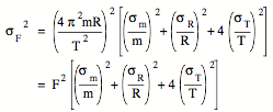
Substituting the numbers into this equation, we obtain the following value for the standard deviation:

sF = 0.07 N

The final answer is therefore:

      F = 7.09 ± 0.07 N

 

Example:  Measuring a spring constant

A spring was purchased.  According to the manufacturer, the spring constant k of this spring equals 0.103 N/cm.  For a spring, the following relation holds: F = k x, where F is the force applied to one end of the spring and x is the elongation of the spring.  A series of measurements is carried out to determine the actual spring constant.  The results of the measurements are shown in Figure 3 and in Table 1.

Table 1.  Results of a series of measurements of the spring constant.

Since F/x = k, the last column in Table 1 shows the measured spring constant k.  Since k is independent of F and x, our best estimate for k will be the average of the values shown in the last column of Table 1:

      k = 0.098 N/cm

Figure 4 shows the ratio of F and x as a function of the applied force F.  The solid line shows the calculated spring constant of 0.098 N/cm.

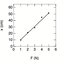
Fig.3. Measured displacement x as a function of the applied force F.  The line shows the theoretical correlation between x and F, with a spring constant obtained in the analysis presented below.

The standard deviation of the measured spring constant can be easily calculated:

sk = 0.006 N/cm

Statistical theory tells us that the error in the mean (the quantity of interest) is not likely to be greater than s/N1/2.  In this case, N = 5, and the error in k is unlikely to be larger than 0.003 N/cm.  The difference between the measured spring constant and the spring constant specified of the manufacturer is 0.005 N/cm, and it is therefore reasonable to suspect that the spring does not meet its specifications.

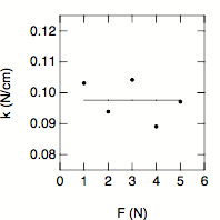
Fig.4. Calculated ration of F and x as a function of the applied force F. The line shows the average spring constant obtained from these measurements.

The standard deviation of the measured spring constant can be easily calculated:

sk = 0.006 N/cm

Statistical theory tells us that the error in the mean (the quantity of interest) is not likely to be greater than s/sqrt(N).  In this case, N = 5, and the error in k is unlikely to be larger than 0.003 N/cm.  The difference between the measured spring constant and the spring constant specified of the manufacturer is 0.005 N/cm, and it is therefore reasonable to suspect that the spring does not meet its specifications.

 

Weighted mean

The calculation of the mean discussed so far assumes that the standard deviation of each individual measurement is the same.  This is a correct assumption if the same technique is used to measure the same parameter repeatedly.  However, in many applications it is necessary to calculate the mean for a set of data with different individual errors.  Consider for example the measurement of the spring constant discussed in the previous Section.  Suppose the standard deviation in the measurement of the force is 0.25 N and the standard deviation in the measurement of the elongation is 2.5 cm.  The error in the calculated spring constant k is equal to:

     

For the first data point (F = 1.0 N and x = 9.7 cm) the standard deviation of k is equal to 0.037 N/cm.  For the last data point (F = 5.0 N and x = 51.5 cm) the standard deviation of k is equal to 0.007 N/cm.  We observe that there is a substantial difference in the standard deviation of k obtained from the first and from the last measurement.  Clearly, the last measurement should be given more weight when the mean value of k is calculated.  This can also be illustrated by looking at a graph of the measured elongation x as a function of the applied force F (see Figure 5).  The theoretical relation between x and F predicts that these two quantities have a linear relation (and that x = 0 m when F = 0 N).  The data points shown in Figure 5 have error bars that are equal to ± 1s.  The dotted lines in Figure 5 illustrate the range of slopes that produces a linear relation between x and F that does not deviate from the first data point by more than 1 standard deviation.  The solid lines illustrate the range of slopes that produces a linear relation between x and F that does not deviate from the last data point by more than 1 standard deviation.  Obviously, the limits imposed on the slope (and thus the spring constant k) by the first data point are less stringent than the limits imposed by the last data point, and consequently more weight should be given to the last data point.

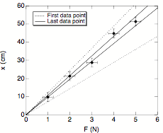Fig.5.   Measured elongation x as a function of applied force F.  The various lines shown in this Figures are discussed in the text.

The correct way of taking the weighted mean of a number of values is to calculate a weighting factor wi for each measurement.  The weighting factor wi is equal to

     

where si is the standard deviation of measurement # i.  The weighted mean of N independent measurements yi is then equal to

     

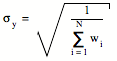
where yi is the result of measurement # i.  The standard deviation of the weighted mean is equal to

     

For the measurement of the spring constant we obtain:

k = 0.095 N/cm

and

sk = 0.004 N/cm

The results obtained in this manner are slightly different from those obtained in the previous section.  The disagreement between the measured and quoted spring constant has increased.