Energy and Momentum of Collisions

Relating Momentum and Kinetic Energy to Can Deformation

Trip and Zach

Passenger Cart Collisions

(4/14/03-4/30/03)

Abstract

The purpose of the passenger cart collisions was to use video imaging to analyze inelastic collisions. This enabled us to develop or refute any relationship between conservation of momentum and kinetic energy and can deformation from the collisions of the carts. Our main results indicated that there definitely was a relationship between can deformation and loss of kinetic energy in the collisions.

Theory

The underlying principals behind the actual collisions that took place existed in the theories of conservation of linear momentum and kinetic energy and also in can deformation magnitude. As a general assumption about the deformation of the cans attached to the carts, we operated with two rules in mind when analyzing our data: 1) the energy required to deform the can(s) is proportional to the deformation and 2) that energy is also proportional to the square of the deformation.

The theory for conservation of linear momentum in relation to our two passenger carts is as follows:

m₁v₁ + m₂v₂ = m₁v₁’ + m₂v₂’

or

(m₁v₁ + m₂v₂) – (m₁v₁’ + m₂v₂’) = 0

The theory states that the product of an object’s initial mass and velocity added to that of the second object’s initial state should equal the sum of the final values (or “after-collision” state) of both objects.

With respect to kinetic energy release, the following formula depicts how that value is calculated:

E_deformation = Change in K_E

Change in K_E = ABS[(½ m₁v₁² + ½ m₂v₂²) - (½ m₁v₁^2’ + ½ m₂v₂^2’)]

Thus, the energy of deformation is equivalent to the change in kinetic energy from initial kinetic to final kinetic states during the collisions.

Experiments

In our experiments we used two students, two passenger collision carts with can mounts, more than 150 cans for 18 trials (CAN FROM THE SAME MANUFACTURER), two meter sticks, a scale, a camcorder, and VideoPoint video analysis software. The experiment was setup up with a collision point (or reference point) picked at an arbitrary location along a sidewalk. From this point, lines were drawn with chalk the same distance away in opposite directions, and then one more set another identical distance beyond that. This guide gave each cart pusher a precise location of where to start pushing the cart and where to let go before the cart and person coasted to the central collision spot. For each collision, the passenger’s mass was noted and the deformation of the cans was measured can-by-can and then tabulated.

For each collision, the video camera recorded the people in it, the trial number, and the collision itself. This video was then spliced and converted to 18 separate movies (one for each run), which were then burned to a CD and analyzed with VideoPoint software. During the analysis, a crucial screen calibration of a known distance was made. This known distance was the measured length from the front to back wheels of a cart. After calibration, the video could be broken down into the two objects and their tracked movement between all frames. This ball-park selection method provided the data for which the rest of the experiment was constructed upon.

Data Analysis

Taking Measurements

The actual data plots taken from the video recordings were applied by hand in a “best-guess” fashion based on our ability to follow the same pixel through all frames. Of these data plots, the ones we used to form our “initial” and “final” calculations for velocity were located in sets of 4 or 5 points just before and just after the collision, respectively, as illustrated in the following graph:

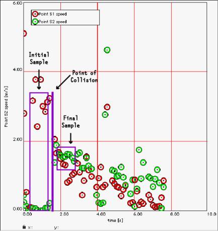
Figure 1: Run 2 (Trip Moving, Zach Still) Velocity Plot

It was easy to pick a collision point based on where the data points jumped up or down to a new velocity value. From this location, one could project forward and backward about five points to obtain an average value for both initial and final velocity of the left and right carts.

Determining Errors

Our error determination came from comparing different measurements taken by each person involved in their respective run. Four separate measurements were analyzed for error: V_i left, V_i right, V_f left, and V_f right. For example, the average values that I calculated me for Run 2 were compared with Zach’s average values and the “plus or minus error” for that particular measurement was just half of the difference between each set of measurements. The following table shows the velocity errors in their entirety:

PLUS/MINUS ERROR
Run	Vi L	Vi R	Vf L	Vf R
1	0.25	0.15	0.27	0.05
2	0.26	0.10	0.19	0.03
3	0.27	0.28	0.13	0.09
4	0.40	0.03	0.07	0.07
5	0.00	0.25	0.01	0.13
6	0.38	0.21	0.36	0.26
7	0.00	0.48	0.14	0.12
8	0.00	0.00	0.00	0.00
9	0.15	0.32	0.04	0.07
10	1.43	0.00	1.00	0.91
11	0.00	0.08	0.72	0.24
12	0.29	1.05	0.53	0.01
13	0.00	0.00	0.00	0.00
14	0.43	0.30	0.10	0.04
15	1.10	0.23	0.26	0.28
16	0.23	0.33	0.44	0.60
17	0.39	0.88	0.07	0.12
18	0.08	0.40	0.14	0.95

Figure 3: Velocity Error Calculations

As Figure 3 shows, our errors were as extreme as ± 1.5 m/s and as small as ± 0.01 m/s. However, on average, our error was normally between

± 0.1 m/s and ± 0.5 m/s, which for all intensive purposes is acceptable for the level of precision we could expect from the analog video camcorder we were using, coupled with the manual data plotting in VideoPoint (Please see the external Excel file for full access to the numbers used in the Figure 3 calculations). I was important to note that Runs 8 and 13 were nullified due to a complete miss in Run 8 and a crash in Run 13.

Examining Conservation of Momentum

In our experiment, it was necessary to use object mass (in our case it was just the person’s mass since both carts were identical in mass) and calculated average velocity to produce average values for momentum. Excel formulas were used to extrapolate a value of momentum (P) for each side (left and right) and for each state (initial and final). The following spreadsheet sample provides insight into how the momentum data was produced:

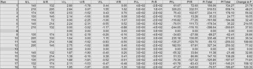
Figure 4: Average Momentum Value Table

It was clear from looking at P_i total and P_f total (the last two columns) and then looking at Change in P (the last column) in Figure 4 that conservation, although not proven with 100% accuracy here, was conserved. One could assume that by looking at how large the values are for difference in momentum that momentum might not be conserved. Below are the last three columns in the Figure 4’s data table:

RUNS	Pi Total	Pf Total	Change in P
1	156.06	134.27	21.79
2	610.53	658.74	48.21
3	234.11	178.10	56.02
4	35.33	24.77	10.55
5	-161.68	-194.08	32.40
6	-179.34	35.22	214.55
7	-398.64	-360.81	37.83
8	0.00	0.00	0.00
9	-89.27	-62.41	26.86
10	335.48	371.83	36.34
11	-56.13	-256.03	199.90
12	327.34	250.32	77.02
13	0.00	0.00	0.00
14	11.38	-21.48	32.86
15	147.10	138.28	8.82
16	-125.86	-197.67	71.81
17	12.91	-145.21	158.12
18	-76.57	-196.87	120.30

Figure 5: Average Momentum Calculations

However, a larger Change in P was justified by larger values of momentum in most cases, so the differences were all of the same proportions across all 18 runs. There were exceptions to the trend (see Runs 6, 11, 17, 18) and these values were most likely obtained because of systematic error in the way that the VideoPoint data were manually plotted by the respective participants.

Examining Conservation of Kinetic Energy

We expected that there would be a loss of kinetic energy (kinetic energy is released in the inelastic collision through the crushing of the cans and also through friction). The following data table illustrates our kinetic energy calculations based on our average value velocities used to obtain momentum:

Ki L	Ki R	Kf L	Kf R	Ki Total	Kf Total	Change in Ke
547.82	210.23	13.58	19.97	758.05	33.55	-724.50
846.89	0.49	253.39	269.67	847.38	523.06	-324.32
555.78	156.67	16.35	39.04	712.45	55.39	-657.06
296.84	201.36	0.51	0.60	498.20	1.11	-497.09
0.00	181.52	62.03	41.45	181.52	103.48	-78.04
352.41	568.94	20.91	29.17	921.35	50.07	-871.27
0.00	601.95	142.51	51.11	601.95	193.62	-408.33
0.00	0.00	0.00	0.00	0.00	0.00	0.00
313.47	415.36	4.49	2.19	728.83	6.68	-722.15
274.51	0.00	134.90	71.82	274.51	206.72	-67.79
286.98	279.08	62.67	34.07	566.06	96.74	-469.33
775.33	191.51	81.24	15.75	966.84	96.99	-869.85
0.00	0.00	0.00	0.00	0.00	0.00	0.00
245.44	238.21	10.93	4.34	483.65	15.27	-468.38
125.22	2.60	10.13	17.67	127.82	27.80	-100.02
239.93	344.50	18.33	38.59	584.43	56.93	-527.50
293.28	202.33	14.46	20.00	495.61	34.46	-461.15
136.47	213.56	15.52	101.73	350.03	117.24	-232.78

Figure 6: Average Kinetic Energy Values

Our assumption that kinetic energy was NOT conserved was correct because ALL values of the change in K_E were negative. It was evident that K_i total was larger that K_f total in every case.

Analyzing Error for Both Momentum and Kinetic Energy Change

In both series of calculations, kinetic energy and momentum value for initial left and right and final left and right were added to get initial and final totals so that an overall value of change could be produced. The table below shows minimum and maximum versions of these values; they were calculated from subtracting and adding the plus/minus velocity errors to and from the original average values to get two more tables of identical labels (See attached excel file for complete calculations):

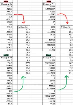
Figure 7: Min/Max-Generated Error for K_E and P

The error in K_E calculations was obtained by halving the absolute difference of the min and max values; P error was reached in the same manner. The K_E error ranged from about ± 50 J to ± 300 J. The error for P was anywhere from ± 7 kg m/s to ± 150 kg m/s. All runs were performed in at least slightly different conditions, and at most at completely different speeds. This fact accounts for the varying magnitude and value of the errors between the runs and makes it irrelevant to compare them beyond the fact that they are all in proportion to their respective values of momentum and kinetic energy, as was explained in Figure 5.

Relating Can Deformation to Kinetic Energy Loss

All can deformation values were measured in centimeters of defamation from a full “normal” length of 10.4 cm. The following table shows the individual can defamation values and then the TOTAL deformation in bold:

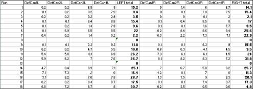
Figure 8: Can Deformations

We observed that, for example, in Run 1, where both objects were moving at each other at similar opposite velocities, the total deformation of the cans was similar, too, in value. However, in Run 2 and others alike where one objects is moving and hits another stationary object with zero velocity, the deformation of the cans is drastically different. To us this suggested that there was a direct, linear relationship between the loss of kinetic energy and the magnitude of can deformation.

We started out with total can defamations from the left and right, so it only made sense to add left and right defamations to obtain a grand total to compare with Change in K_E. From our theory (See Page 1) we knew that defamation was proportional to kinetic energy and kinetic energy squared. So in order to create a graph that displayed a linear relationship, we would have to experiment with the following mathematically-manipulated values of K_E:

Run	LEFT total	RIGHT total	TOTAL Def	Ke	Ke^2
1	15.2	14.1	29.3	-724.5	5.2E+05
2	8.4	15.4	23.8	-324.3	1.1E+05
3	3.5	2.1	5.6	-657.1	4.3E+05
4	15.4	17.0	32.4	-497.1	2.5E+05
5	9.6	9.5	19.1	-78.0	6.1E+03
6	22.0	25.6	47.6	-871.3	7.6E+05
7	2.2	22.9	25.1	-408.3	1.7E+05
8	0.0	0.0	0.0	0.0	0.0E+00
9	11.8	15.5	27.3	-722.2	5.2E+05
10	10.6	9.5	20.1	-67.8	4.6E+03
11	26.2	24.0	50.2	-469.3	2.2E+05
12	26.7	31.8	58.5	-869.9	7.6E+05
13	0.0	0.0	0.0	0.0	0.0E+00
14	25.1	25.7	50.8	-468.4	2.2E+05
15	16.4	11.3	27.7	-100.0	1.0E+04
16	26.7	26.1	52.8	-527.5	2.8E+05
17	17.5	17.3	34.8	-461.2	2.1E+05
18	30.7	4.8	35.5	-232.8	5.4E+04

Figure 9: Comparing Total Deformation to K_E and K_E²

Once we had the K_E and K_E² values tabulated with total deformation, we could set up a visual representation to see if indeed there was or was not a linear relationship in our data:

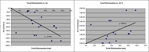
Figure 10: Def. Total/K_E Graphical Analysis

The graphical representation of the data when looking at total deformation versus K_E indicates a probable linear but indirect relationship. As total deformation of the cans increases, the amount of kinetic energy gets increasingly negative (more is released). When plotted against K_E², however, there is a linear but direct relationship. These graphs, although there are some extreme outlier data points, do illustrate a pattern that suggests a linear relationship.

Conclusion

We had several underlying theories governing the behavior of the carts. The first was the conservation of momentum. Our data suggested without reasonable double that momentum was conserved. The second theory, conservation of kinetic energy, was disproved. As expected, in all runs kinetic energy was released (negative) because there was defamation in at least 1 can every time (which was obvious from the inelastic behavior). The last theory, that of the linear relationship between total deformation and kinetic energy, was an indirect one based on the sign value for kinetic energy decreasing (getting increasingly negative) as deformation went up. That was also expected and backed up the assumption that the more the cans were crushed, the more kinetic energy had to have been released.

Remarks

The experiment itself was a fascinating conclusion to the weeks of work did on collisions and the conservation laws. I was impressed with how simple the actual trials were compared to the wealth of data and variables that lay beneath the collisions. This lab offered not just a recapitulation of the concepts we already were familiar with, but made us think about what those principals meant abstractly.