Scientific
Method
February 26 – March 17, 2003 ˜
PHYSICS BY INQUIRY
By: Dan Bobkoff and Kelly McNamee
Abstract
In this series of experiments, we formulated theories from the results of a collection of data. In each of these experiments we changed certain variables to develop an array of data that was interpreted to find one inclusive theory. Unlike last time, the theory came from the experiments, not as a pre-existing hypothesis.
Theory
Often it is not possible to predict the outcomes of scientific experiments. In these such instances, the theory is developed through repeated experimentation. In these three experiments, we analyzed acceleration with a number of variables to determine theories such as that mass doesn’t affect acceleration, and acceleration is directly affected by the height of the track. We found three mathematical equations to explain each of the three experiments and thus develop a theory.
Experiment
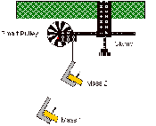
In experiment P13, we set up the smart pulley off the edge of the table as indicated in the diagram below. We hung one mass on Mass 1 and a slightly heavier mass on Mass 2. We moved the heavier mass upwards and the smaller mass downwards so that it almost touched the floor. We then let go of the heavier mass. We changed the masses of M1 and M2 by taking mass from one and adding it to the other. By doing this we changed the net force without altering the total mass. Next, we changed the total mass but kept the net force the same by adding the same amount of additional mass to both hangers.
For experiment P09a, as shown below, we used a photogate and a picket fence to measure the velocity of a cart on a track which was elevated to differing heights and a pulley connected to the cart which was weighed down by differing masses. To do this, we raised one end of the track to a height of 0.1 meters, and at this height, did five different measurements changing the weight from 50 to 100 to 150 to 200 to 250 grams. We then did these five measurements at five additional heights (0.15, 0.2, 0.25, 0.3, 0.35m).
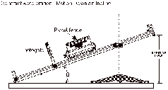
Then, in experiment P10a, the set up was similar to that of P09a, except that there was no weight attached to the cart and we used two photogates spaced at varying distances from each other. First, we raised one end of the track to 0.2m. The photogates were placed at the 0.25m mark and 0.55 (looking away from the beginning of the cart which was poised at the top of the track). In the first run, there was no weight added to the cart, however we did two more sets of runs, adding first, one block of weight, and then, two blocks of weight. We repeated these exact measurements, but we changed the photogates to be spaced at 0.35m and 0.65m and then to 0.45m to 0.75m. Then, we did these exact measurements changing the heights to 0.15m and 0.1m.
Data
Analysis
In experiment P13, we experimented usin constant total mass and constant net force (as said in the Experiments section). Based on our observations of the change in acceleration due to the change in net force we were able to create a theory: Acceleration= C(M1-M2)g/(M1+M2). We then used this relation to compare experimental acceleration to theoretical acceleration (as seen in the table below).
|
Trial |
M1 (kg) |
M2 (kg) |
a exp
(m/s^2) |
M1 + M2
(kg) |
a theory
(m/s^2) |
% diff |
|
1 |
75 |
15 |
3.62122222 |
90 |
6.533333333 |
0.44573129 |
|
4 |
60 |
30 |
1.79215 |
90 |
3.266666667 |
0.45138265 |
|
7 |
40 |
50 |
0.4818 |
90 |
-1.088888889 |
1.44246939 |
|
10 |
20 |
70 |
3.006894737 |
90 |
-5.444444444 |
1.55228679 |
As seen in this table, although our experimental and theoretical accelerations may seem very different the % difference is negligible. Therefore our theory seems successful.
In experiment P09a, we looked at our data and came up with the following equation to explain the found acceleration: Acc=Mgsinq-mg/M+m. We then made sure this equation worked by graphing Experimental Acceleration vs. Calculated Acceleration.
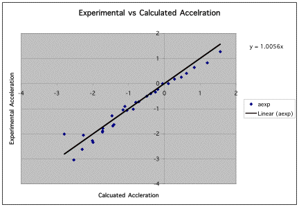
Since the slope of this line is very close to 1 it shows that our theory is successful.
The following table shows all of our data. Like the graph above, this table shows that our equation is accurate by showing the percent difference between calculated and experimental acceleration.
|
run |
m |
M |
H |
sin(theta) |
acalc |
aexp |
daexp |
|
1 |
55 |
496 |
10 |
0.08230453 |
-0.2521491 |
-0.3406667 |
0.0205 |
|
2 |
105 |
496 |
10 |
0.08230453 |
-1.0464795 |
-1.0693333 |
0.229 |
|
3 |
155 |
496 |
10 |
0.08230453 |
-1.7187929 |
-1.7893333 |
0.5335 |
|
4 |
205 |
496 |
10 |
0.08230453 |
-2.2951985 |
-2.6246667 |
0.967 |
|
5 |
255 |
496 |
10 |
0.08230453 |
-2.7948524 |
-2.0146667 |
0.6315 |
|
6 |
55 |
496 |
15 |
0.12345679 |
0.11088705 |
0 |
0 |
|
7 |
105 |
496 |
15 |
0.12345679 |
-0.713646 |
-0.7246667 |
0.0655 |
|
8 |
155 |
496 |
15 |
0.12345679 |
-1.4115226 |
-1.6366667 |
0.215 |
|
9 |
205 |
496 |
15 |
0.12345679 |
-2.0098448 |
-2.2796667 |
0.278 |
|
10 |
255 |
496 |
15 |
0.12345679 |
-2.528497 |
-3.0473333 |
0.092 |
|
12 |
55 |
496 |
20 |
0.16460905 |
0.47392321 |
0.25266667 |
0.0785 |
|
13 |
105 |
496 |
20 |
0.16460905 |
-0.3808125 |
-0.4023333 |
0.1045 |
|
14 |
155 |
496 |
20 |
0.16460905 |
-1.1042524 |
-0.9103333 |
0.6195 |
|
15 |
205 |
496 |
20 |
0.16460905 |
-1.7244912 |
-1.895 |
0.3605 |
|
16 |
255 |
496 |
20 |
0.16460905 |
-2.2621416 |
-2.0566667 |
0.511 |
|
17 |
55 |
496 |
25 |
0.20576132 |
0.83695936 |
0.64266667 |
0.1395 |
|
18 |
105 |
496 |
25 |
0.20576132 |
-0.047979 |
-0.0026667 |
0.122 |
|
19 |
155 |
496 |
25 |
0.20576132 |
-0.7969822 |
-0.7463333 |
0.1525 |
|
20 |
205 |
496 |
25 |
0.20576132 |
-1.4391375 |
-1.6886667 |
0.43 |
|
21 |
255 |
496 |
25 |
0.20576132 |
-1.9957861 |
-2.344 |
0.297 |
|
22 |
55 |
496 |
30 |
0.24691358 |
1.19999552 |
0.82566667 |
0.2205 |
|
23 |
105 |
496 |
30 |
0.24691358 |
0.28485446 |
0.17533333 |
0.0035 |
|
1a |
155 |
496 |
30 |
0.24691358 |
-0.4897119 |
-0.5026667 |
0.1835 |
|
2a |
205 |
496 |
30 |
0.24691358 |
-1.1537838 |
-1.05 |
0.1815 |
|
3a |
255 |
496 |
30 |
0.24691358 |
-1.7294307 |
-1.9306667 |
0.259 |
|
4a |
55 |
496 |
35 |
0.28806584 |
1.56303167 |
1.27333333 |
0.468 |
|
6a |
105 |
496 |
35 |
0.28806584 |
0.61768794 |
0.409 |
0.093 |
|
7a |
155 |
496 |
35 |
0.28806584 |
-0.1824417 |
-0.229 |
0.06 |
|
8a |
205 |
496 |
35 |
0.28806584 |
-0.8684302 |
-1.0213333 |
0.178 |
|
9a |
255 |
496 |
35 |
0.28806584 |
-1.4630753 |
-1.2843333 |
0.7685 |
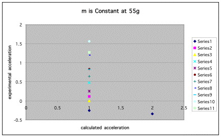
As the table below shows, mass does not play a part in the acceleration of the cart. Clearly, the data points create a vertical line, telling us that the mass was insignificant.
As this next table shows, the incline (sinq) does play a role in the acceleration of the cart. As you can see, the data points create a line through zero with a slope very near 1.
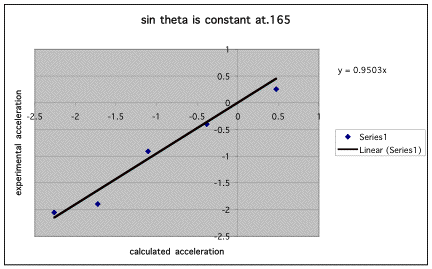
All of these graphs and tables tell us that our equation is successful.
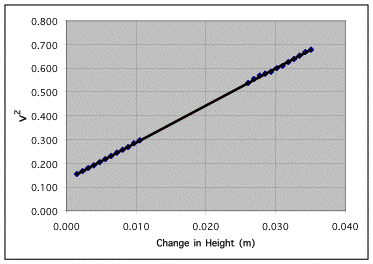
In experiment P10a, we again used our data to form yet another equation: (h0-h1) vs (v0-v1)2. We found that this was the only equation that was linear. Before we found this equation, we had to determine if mass affected acceleration or not. In the graph below, it is shown that mass does not indeed matter. Each color shows a different mass, and in each case, they are the same.
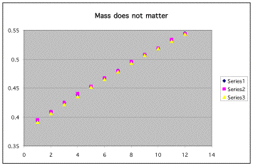
We then put runs 55-56, which had the incline 0.1m and no mass, into the spreadsheet supplied for us. Then, we looked at each graph on the plot sheet to find out which equation was linear. The graph is shown below:
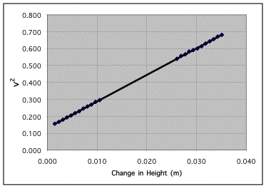
Then, to make sure that this was not anomalous, we did the find same thing with runs 58, 59, and 60. The same equation was linear as shown below.
Conclusion
Through these experiments, we found successful theories to explain our experimental results. The inevitable error in our experiment is indicated by the percent difference in each of the experiments (shown above). Humans are imperfect so we are able to determine that our theories are valid, even if they are not as precise as the theory.
Remarks
The experiments worked as designed for the most part, but P09a, with the weight on the cart and the steep incline, led Kelly to cut her hand as she tried to stop the cart in motion.