Understanding Motion II

Velocity

Trip and Zach

2/3/03 (Photogate/Sensor), 2/5/03 (Video), 2/10/03 (P03)

EXPERIMENTS Photogate I, Video Analysis, P03

Abstract

The purpose of the first Photogate experiment was to illustrate the difference between how the Photogate and the motion sensor measured velocity of an object. The video analysis experiment’s main goal was to show how velocity of an object could be measured by tracking the position and size of an image moving over a set number of frames. Finally, the goal of experiment P03 was to calculate the average velocity of an object based on another set of Photogate measurements.

Our main results were as follows: the Photogate with the picket fence cart was better at measuring instantaneous velocity of an object over a shorter distance and a shorter period of time than the motion sensor for that same object, when viewing video we concluded that tracking pixels through frames was effective at displaying the general trend of velocity of an object which would be too large to measure in a lab, and that the last experiment (P03) clearly demonstrated a relationship between the height of the cart and the velocity of its descent down the track.

Theory

The goal of experiments Photogate I through P03 was to identify the relationships, if any, between different methods of measuring velocity the types of results obtained and then to state from these conclusions the advantages or disadvantages of each method.

Most measurements in these labs we compiled together to produce graphs that had either positive or negative slopes for velocity. The velocity slope is positive when the object measured moves away from the point of reference. Velocity is zero, therefore, when the object is stationary and, consequently, negative whenever the object moves away from the point of reference in the opposite direction.

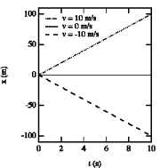
Figure 1: Position as a Function of Time

The slopes shown in the graph above show how velocity can either be positive, zero, or negative, depending on the speed and direction of object movement away from the point of reference.

It is more often than not in these experiments that the change in magnitude of an object’s velocity plays a more significant role in helping us to determine special relationships that does simple sign change (+ or -) in velocity. The following graph illustrates different velocities attained by very different creatures.

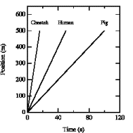
Figure 2: Position versus Time for 3 Animals

At first, the lines on the graph look similar in length and behavior, but when comparing them, there is an obvious difference in steepness of slope. A graph such as this helps to support why we understand that a cheetah is faster than a human, or in our case, why a cart moving from a higher starting point might travel at a greater positive velocity than from a lower starting point.

Key principals tested and compared in the first experiment are average and instantaneous velocity. The average velocity is a calculated value produced by taking the total distance between time between measurements of a moving object and dividing it by the time taken in between those measurements. The instantaneous velocity along any objects path of movement is actually the average velocity in an extremely small time interval. It is important to understand that both are still averages of how we speculate the object is traveling. However, one is better for certain measurements that the other. In theory, instantaneous velocity should be better for measuring an object’s speed and direction at a known place or condition in an experiment. Average velocity is better used to achieve an overall feel for how an object’s movement changes over larger space and a longer period of time.

Experiments

For the Photogate/Motion Sensor experiment, both the motion sensor and Photogates we used in conjunction with a support rod, cart track, cart, picket fence plate, and the Science Workshop interface. In this experiment, 30 total runs were performed using first the motion sensor and then the Photogate to measure instantaneous velocities of the cart as it traveled down the track from a height held constant throughout the measurements.

For the video analysis experiment, both the space shuttle and lunar module videos were analyzed on Mac computers with Science Workshop and a special scaling program that tracked one particular pixel (single unit of light) on the screen through a series of 20 frames of video. A scale for sizing the object size was used for every measurement in order to generate calculations for the distance covered by that object in real space.

For experiment P03, identical equipment used in the first experiment was used here, except for the motion sensor. The measurements were done with the same cart, rolling down a track attached at three specific heights to the side of the support rod. The Photogates were positioned equidistant from the “50 cm” mark on the ruler along the side of the track, and gradually increased from 20 cm apart to 40 cm and then to 60 cm over the course of 9 trials per height, producing a total of 27 trials.

Data Analysis

Example 1 from the Photogate I / Motion Sensor Experiment:

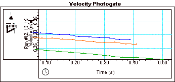
Figure 3: Sample Photogate Readings

The three sample photogate readings were all done with a “picket fence” plate, which was able to generate 12 readings within about 0.5 seconds. The error was kept at < 3 cm/s in the velocity measurements done by the photogate in this time frame.

Example 2 from the Photogate I / Motion Sensor Experiment:

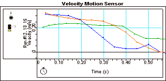
Figure 4: Sample Motion Sensor Readings

As is illustrated above, the motion sensor took the same time sampling of readings, 12 in roughly .5 secs, which translates to about 25 Hz on the motion sensor setting. Its range of error, however, was greater than the photogate at < 7 cm for the average duration of the cart. Both figures clearly illustrate an agreeing trend that the cart, regardless of method used in measurement, reduced its positive velocity over the course of that .5 second margin.

Example from Video Analysis not available.

(Failed to reproduce saved results on home computer).

The video analysis of the space shuttle and lunar module dealt with pixel tracking through multiple frames, or still pictures, played quickly to look as if the object (pixels) were moving. In the case of the shuttle, our best guess at the very end of the wing tip was used to track the shuttle’s movement through space over 20 frames. As a result of keeping this point as constant as possible, Science Workshop was able to calculate a table illustrating a direct relationship between time and velocity of the space shuttle. As time increased, data proved that the shuttle’s positive velocity away from the ground increased as well. Experimental error, although quantitatively unknown, was looked at qualitatively. Even when moving the crosshairs of the mouse to another pixel between 1 and 5 pixels away from the one we have chosen, the margin of error was still well within the relationship we observed.

The lunar module readings added another element to the object’s movement away from the ground (surface of the moon). This entailed the camera zooming out from the module as an attempt to keep the whole vehicle in the frame. We tracked a particular pixel as best we could, but also had to tell Science Workshop to adjust to the size change in every subsequent frame, accordingly. The graph of velocities plotted showed us that after a few frames, the velocity was approaching a constant value. Again, a similar approach to dealing with error was taken with the module video, as we moved our pixel measurement around to simulate the highest possible degree of error, and we still observed the same trend.

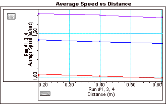
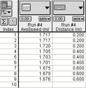
Examples of Average Velocity from Photogate II Experiment P03:

[ A ] [ B ]

Figure 5: a) P03 Average Velocity Results

b) P03 Run #4 Table Values

Experiment P03, part one, measured average speed between photogates set at 20, 40, and 60 cm apart, respectively. After 4 runs (Run 2 was thrown out due to systematic error), we observed a decrease in average speed measured by the photogates over three different runs consisting of starts at 10, 20, and 30 cm off the table were plotted next to each other. For error analysis, the included table of Run #4 values shows how our greatest error between sets of three measurements for the same distance in the same run was always < 3 cm/s (this was true for all other runs as well), which reinforced our conclusion that average speed was decreasing as time increased.

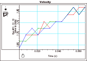
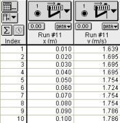
Examples of Instantaneous Velocity from Photogate II Experiment:

[ A ] [ B ]

Figure 6: a) P03 Instantaneous Velocity Results

b) P03 Run #11 Table Values

The second part of experiment P03, as seen above, involved measuring instantaneous velocity with one photogate using the “picket fence” side of the plate (just like in the first Photogate experiment) to take 12 measurements in a time span of < .070 seconds. We found our average experimental error for instantaneous velocity to be < 1.5 cm/s (as illustrated by the table of Run #11). These error plots were well within out observed trend that instantaneous velocity increased over time.

It was extremely important for us to know which picket in the fence to use as our reference point to compare the calculated instantaneous and average velocities to see if our measurements were accurate (in this case, runs at 30 cm off the table from both experiments are being compared). We used plot 6, as the sixth picket matched the line at which the “block” marker starts on the other side of the clear plate used in the average velocity runs. Using Plot #6 (Index 6 in Figure 6b.) we obtained a value of ~ 1.72 M/s instantaneous velocity. When compared with the sixth plot of Figure 5b, we get ~1.70 M/s. The absolute difference was .02 M/s, or 2 cm/s. So, we concluded that our calculated values matched each other with extreme precision given the quality of the photogate readings at distance and close up.

Conclusions

We concluded that there was a crucial relationship between instantaneous and average velocity and whether the motion sensor or photogate was better for measuring each type. The following graph comparison shows three identical runs as recorded by both motion sensor and photogate:

[ A ]

[ B ]

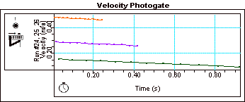
Figure 7: a) Velocity Runs From Photogate

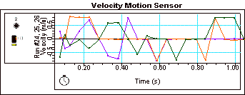
b) Velocity Runs From Motion Sensor

Clearly, the prior data supporting our theory that the photogate was more effective at smaller distances and smaller time intervals is proven correct with an example such as Figure 7. In Part A, one can see that the Photogate modeled a gradual descent of the cart from the same height with three different picket settings to within an error of < .5 cm/s. Part B, it is evident that the motion sensor had problems picking up any change in velocity less than .5 m/s over the same time interval of about 1 second. Its error, respectively, was > 50 cm/s on an average. That is 10 times the error of the photogate! Expectedly, we found that a reverse situation where the time interval was greater than 2 seconds and the distance was approaching 1 meter produced a flipped result in the graphs. This means that the motion sensor excelled at greater distances and longer time intervals as our theory stated.

The shuttle and lunar module recordings could have been sampled and shown at much higher frame-rates and over longer periods of time. This would have given our graph many more data plots and a larger margin to error to accommodate. However, even with the 20-frame samples we used, it was still evident that our theory of the shuttle’s velocity becoming more and more positive and of the lunar module’s velocity approaching zero was protected by a data trend that still accounted for significant errors in our inability to perfectly match the same part of the image with the right pixel every time we re-sampled out image on the next frame.

After examining and comparing them magnitudes of motion sensor versus photogate, we concluded that they equaled each other out overall due to mirrored problems reached after passing their practical limits of measurement (for the photogate it must be < ~0.75 M and < 1 second of time and for the motion sensor the values must be slightly greater). Error in these experiments, therefore, was mostly systematic and rarely accidental, as it was for the last photogate experiment (P03). Error in the video analysis existed equally in our lack of precision with crosshair placement and was compounded by the calculations made by Science Workshop, which assumed every plot was the most accurate attainable value. Once the movie window was increased and pixels blown up, experimental error decreased by a factor of at least 5 times, proving that human error was responsible for making graphs defy certain known physical parameters, such as a mandatory given velocity per unit time.

Remarks

I liked everything about this lab. It was extremely comprehensive and repetitive, almost to the point of being boring, but the experiments were relevant enough to the topic that it did not seem slow at any time in particular.