Understanding Motion I

Distance and Time

Trip and Zach

1/15/03 (P00), 1/17/03 (P00a, P00b, P00c),

1/22/03 (P00a, P00b, P00c), 1/27/03 (P01)

EXPERIMENTS P00, P00a, P00b, P00c, P01, P02

Abstract

The purpose of experiments P00, P00a, P00b, and P00c was to calibrate the motion sensor, test it’s minimum and maximum range and to summarize the relationship of a moving object and the graph of position and time for that object. The purpose of experiment P01 was to explore the relationship of the velocity (the speed and direction) of an object to the graph of that object’s position with the respect to time. The purpose of experiment P02 was to observe and infer information about the relationship between acceleration (the change in velocity over time) and the graph of an object’s acceleration with respect to time.

Our main results were as follows: the sensor’s measurements of distance matched known distances (with acceptable error), the minimum reading for the sensor was .4 M, the maximum was greater than 3.3 M and the reference point, position, speed and direction and acceleration of an object all influenced the shape of a graph of that objects movement with respect to time.

Theory

The goal of experiments P00 through P02 was to draw clear relationships between all measurements of an objects position at a certain time as described by position, velocity, and acceleration.

The most basic measurement, the point of reference, was crucial in making accurate measurements. This is the actual point at which the position value is zero.

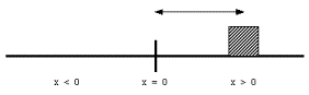
Figure 1: Position Relative to the Reference Point

For example, a set of data could all differ from another set by .5 cm, which in our case was the difference between measuring distances from the front grill of the sensor or the actual plate itself.

The relationship between velocity and position revolves around the speed of the object and in what direction (+ or -) it’s moving. Velocity is positive when moving away from the sensor and negative when moving towards it. Velocity is zero, therefore, when the object is stationary.

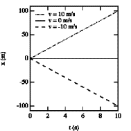
Figure 2: Velocity as a Function of Time

The slopes shown above model how the slope can either be positive, zero, or negative, depending on the speed and direction of movement.

Lastly, acceleration models how velocity (the speed and direction of movement) changes over time. Acceleration in the most complex attribute of movement because it depends upon all of the following to make a single measurement: direction, speed, and if that speed is increasing or decreasing per unit time.

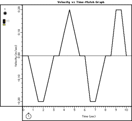
Figure 3: Acceleration as a Function of Velocity versus Time

The acceleration graph depended upon if the object was speeding up or slowing down and, at the same time, in what direction it was doing this.

Experiments

We used a motion sensor, base and support rod, and the Science Workshop interface to record all measurement. The motion sensor was mounted on the stand at a known distance above the table (45.8 cm) and twisted to a position so that the circular sensor was as perpendicular to the table as possible. To calibrate the sensor, we lined up a meter stick below the gold sensor disk and placed a notebook (our object) at the end of the meter stick. For our minimum and maximum measurements we held a notebook in front of the sensor and over the table and walked either towards or away from the sensor, holding the notebook steady and using the meter stick resting on the table below for position reference (Refer to Figures 1 through 3 for explanations as to how we varied our movement to suit each model).

Data Analysis

Example from the P00 Calibration Experiment:

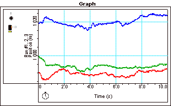
Figure 4: Run Data From P00

We were able to estimate accurately measure the distance of 1 meter to an error of < 4 cm when we looked at our largest and smallest graphs.

Example from the P00a/b/c Minimum Experiments:

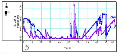
Figure 5: P00a Minimum Results

Figure 5 illustrates how we used two identical movements from about 1 meter away from the sensor in towards the it and back out again to test the minimum reading. We obtained a value of exactly .4 M with an error of < 1 cm. We did not draw any relationship between the requency of the sensor’s pulses and the minimum range of the sensor in P00a, P00b, or P00c, as they were all identical.

Example from the P00a/b/c Maximum Experiments:

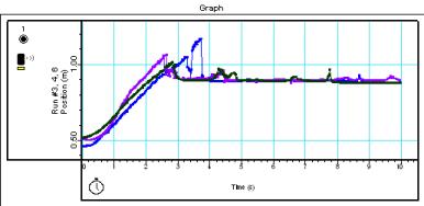
Figure 6: P00b Maximum Results

Our maximum readings were taken at the point that an even slope ceased, right before an observed “drop-off” in the graph. We were able to approximate P00b’s maximum to be 1.04 M, with an error of < .3 cm. The calculated value for P00a was .50 M, with an error of < .2 cm and the P00c maximum was > 3.5 M. (P00c limited us to a maximum of the distance between the sensor and the next computer on the table). The varying results here, we postulated, were because of the varying frequencies of sound pulses coming from the sensor. The higher the frequency, we thought, the smaller the maximum range would be. Our postulate was proven true, based on a 120 Hz reading for a .50 M maximum, 60 Hz reading for a 1.04 M max, and 20 Hz reading for > 3.5 M maximum.

Example from the P01 Velocity Modeling Experiment:

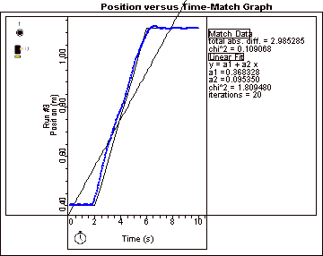
Figure 7: P01 Velocity Matching

Our attempt to model velocity produced a total absolute difference of 2.985 and a chi² value of 0.1. This run clearly proved our theory that an object had to remain stationary for 2 seconds to produce a slope of zero, had to move away at a constant rate for 4 more seconds, and remain stationary again for the remaining 4 to match the model.

Example from the P02 Acceleration Modeling Experiment:

Please see attached printout sheet marked “Figure 8: Acceleration Matching.”

The acceleration results we obtained produced a total absolute difference of 20 and a chi² value of 3.5. We attributed the rise in both numbers to be a result of how the program measured acceleration. Since Science Workshop used the velocity position measurements at t=a and t=b to compute a single acceleration measurement, the experimental error could have been so great and the velocity measurements so close that Science Workshop would have known how to plot certain acceleration readings, thus making large “blips” in the readings and increasing the experimental error.

Conclusions

We concluded from our experiments that the sensor, in the mid to high frequencies (from 60 Hz to 120 Hz and higher) was accurate at measuring distances to within an error or < 5 cm. Based on the meter scale we were using in Science Workshop, this was very acceptable. The sensor excelled at measuring all minimums, therefore, and all but one maximum (where we were limited by space in the room).

Velocity was easily modeled with a middle-range frequency because the only variables we had to work with was direction and speed. Our absolute difference for our velocity model (2.985) was very acceptable, considering our lack of ability in making every movement perfectly smooth. The acceleration model, however, gave us an absolute difference of 20, which previously illustrated showed how the error we were experiencing in all other measurements affected our results here more than anywhere else.

Sources of error, we concluded, were attributed to only a few variables. The first was the object itself. In our case it was a notebook held in place by a person’s hands. Wavering of the notebook and mistakes in walking probably produced our greatest errors. Second, the sensor’s cone of reception made accurate readings more difficult as one walked further away from the sensor. The cone was biggest at that point and could have picked up on objects other than our notebook. Finally, frequency played a larger part in making our errors consistently visible. For example, P00b’s 60 Hz measurement always dropped off between 1.01 and 1.11 M due to the increased rate at which signals were simultaneous coming in and out of the sensor when compared to a 20 Hz sampling in P00c, where a maximum of > 3.5 M was recorded.

Remarks

The only criticism I have for the procedure, as explained in the lab manual, is that an explanation of the pros and cons for measuring distances with one’s body versus an inanimate object being held my hand was lacking. If I had a second chance to do this experiment, I would attempt all measurements with a cleared path the whole length of the room. This would allow for better approximations of a maximum sensor range and also for easier attempts at modeling acceleration, as I could use a lower frequency over a larger space. That way I could spread out and exaggerate my movements, with a little more room for experimental error, over several meters, rather than doing them in the space of a .5 M over a table with a notebook.

Overall, though, the experiment was very clean and straightforward in helping me to visualize what position, velocity, and acceleration mean when looking at a graph.