Atwood's Machine
Concept: Newton's Laws
Time: 45 m
SW Interface: 700
Macintosh® file: P13 Atwood's Machine
Windows® file: P13_ATWD.SWS
EQUIPMENT NEEDED
- Science Workshop Interface
- table clamp, universal
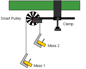
- Smart Pulley
- thread
- mass set & hanger (two)
PURPOSE
The purpose of this laboratory activity is to study the relationship
between force, mass, and acceleration using an Atwood's Machine apparatus.
Based on the measurements you carry out as part of this experiment you will
predict the acceleration of the system, in terms of the masses connected
to the Atwood machine.
THEORY
The acceleration of an object depends on the net applied force, and the
mass. In an Atwood's Machine, the difference in weight between two hanging
masses determines the net force acting on the system of both masses. This
net force accelerates both of the hanging masses; the heavier mass is accelerated
downward, and the lighter mass is accelerated upward.
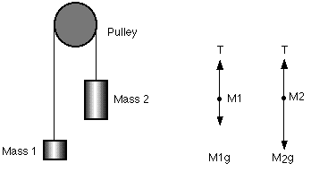
In the free body diagram of the Atwood's machine, T is the tension in
the string, M1 is the lighter mass, M2 is the heavier mass, and g is the
acceleration due to gravity. Assuming that the pulley has no mass, the string
has no mass and doesn't stretch, and that there is no friction, the net
force on M1 is the difference between the tension and M1 g (T>M1 g).
The net force on M2 is the difference between the tension and M2 g (T<M2
g).
PROCEDURE
For this activity, the Smart Pulley will measure the motion of both masses
as one moves up and the other moves down. The Science Workshop program
calculates the changing speed of the masses as they move. A graph of speed
and time reveals the acceleration of the system.
PART I: Computer Setup
- Connect the Science Workshop interface to the computer, turn on the interface,
and turn on the computer.
- Connect the stereo phone plug of the Smart Pulley to Digital Channel 1 on
the interface.
- Open the Science Workshop document "P13 Atwood's Machine" which
is located in your handout folder. The document opens with a Graph display
of Velocity (m/sec) versus Time (sec).
- For quick reference, see the Experiment Notes window. To bring a display
to the top, click on its window or select the name of the display from the
list at the end of the Display menu. Change the Experiment Setup window by
clicking on the "Zoom" box or the Restore button in the upper right
hand corner of that window. The "Sampling Options..." are: Periodic
Samples rate = Fast at 10 Hz, Digital Timing rate = 10000 Hz, and Start Condition
= Ch. 1, Low ("Photogate Blocked").
PART II: Sensor Calibration and Equipment Setup
- You do not need to calibrate the Smart Pulley.
- Mount a clamp to the edge of a table. Place the Smart Pulley in the clamp
so that the Smart Pulley's rod is horizontal.
- Use a piece of thread about 10 cm longer than the distance from the top
of the pulley to the floor. Place the thread in the groove of the pulley.
- Fasten mass hangers to each end of the thread. You can fasten the mass hangers
to the thread by wrapping the thread four or five turns around the notched
area of the mass hanger.
- Place about 100 grams of mass on one mass hanger and record the total mass
as M1. Be sure to include the 5 grams from the mass hanger in the total mass.
Place slightly more than 100 grams on the other hanger. Record this total
mass as M2.
- Move the heavier of the two masses upward until the lighter mass almost
touches the floor. Hold the heavier mass to keep it from falling. Turn the
pulley so that the photogate beam of the Smart Pulley is unblocked (the red
light-emitting diode (LED) on the photogate does not light).
PART IIIA: Data Recording Constant Total Mass
- Click the "REC" button. Let the heavier mass fall. Data recording
will begin when the photogate beam of the Smart Pulley is blocked.
- Click the "STOP" button to end data recording just before the
heavier mass reaches the floor. Don't let the upward moving mass hit the
Smart Pulley! "Run #1" will appear in the Data list in the Experiment
Setup window.
- Change the relationship between M1 and M2 by removing mass from one hanger
and adding it to the other. This allows you to change the net force without
changing the total mass.
- Repeat the data recording procedure using different combinations of M1 and
M2. Record the mass of M1 and M2 for each combination. Change the net force
each time, but keep the total mass constant.
PART IIIB: Data Recording Constant Net Force
- Arrange the masses as they were for the beginning of Part IIIA. Now, change
the total mass but keep the net force the same as for the first run in Part
IIIA. To do this, add exactly the same amount of additional mass to both mass
hangers. Make sure that the difference in mass is the same as it was for
the beginning of Part IIIA.
- Record your new values for M1 and M2.
- Record data as in Part IIIA.
- Repeat the process several times. Change the total mass each time but keep
the net force constant.
ANALYZING THE DATA
Data Table #1: Constant Total Mass
|
Trial
|
M1 (kg)
|
M2 (kg)
|
a exp (m/s^2)
|
M1 + M2 (kg)
|
a theory (m/s^2)
|
% Diff.
|
| 1 |
|
|
|
|
|
|
| 2 |
|
|
|
|
|
|
| 3 |
|
|
|
|
|
|
| 4 |
|
|
|
|
|
|
| 5 |
|
|
|
|
|
|
| 6 |
|
|
|
|
|
|
| 7 |
|
|
|
|
|
|
| 8 |
|
|
|
|
|
|
| 9 |
|
|
|
|
|
|
| 10 |
|
|
|
|
|
|
| 11 |
|
|
|
|
|
|
| 12 |
|
|
|
|
|
|
| 13 |
|
|
|
|
|
|
| 14 |
|
|
|
|
|
|
| 15 |
|
|
|
|
|
|
Data Table #2: Constant Net Force
|
Trial
|
M1 (kg)
|
M2 (kg)
|
a exp (m/s^2)
|
M1 + M2 (kg)
|
a theory (m/s^2)
|
% Diff.
|
| 1 |
|
|
|
|
|
|
| 2 |
|
|
|
|
|
|
| 3 |
|
|
|
|
|
|
| 4 |
|
|
|
|
|
|
| 5 |
|
|
|
|
|
|
| 6 |
|
|
|
|
|
|
| 7 |
|
|
|
|
|
|
| 8 |
|
|
|
|
|
|
| 9 |
|
|
|
|
|
|
| 10 |
|
|
|
|
|
|
| 11 |
|
|
|
|
|
|
| 12 |
|
|
|
|
|
|
| 13 |
|
|
|
|
|
|
| 14 |
|
|
|
|
|
|
| 15 |
|
|
|
|
|
|
QUESTIONS
- Based on your observations in this experiments, try to determine a relation
between the acceleration of the system, and the masses attached to the pulley.
- Use this relation to compare the experimental acceleration with your theoretical
acceleration. Determine the percentage difference. What are some reasons that
would account for the percentage differences?
- Use your theoretical correlation to predict the outcome of new measurements.
Verify these predictions by carrying out these new measurements.
© Frank L. H.
Wolfs, University of Rochester, Rochester, NY 14627, USA
Last updated on
Saturday, February 23, 2002 19:36