Acceleration of a Dynamics Cart II
(Motion Sensor)
Concept: Newton's Laws
Time: 30 m
SW Interface: 700
Macintosh® file: P10 Cart Acceleration II
Windows® file: P10_CAR2.SWS
EQUIPMENT NEEDED
- Science Workshop Interface
- dynamics cart
- motion sensor
- protractor
- adjustable feet, track
- track, 1.2 meter
PURPOSE
In this laboratory activity you will investigate the acceleration of
a cart as it moves up and down an inclined plane. You will determine whether
the acceleration of the cart is constant.
THEORY
If a cart moves on a plane that is inclined at an angle [theta], the
component of force acting on the cart in a direction that is parallel to
the surface of the plane is mg sin [theta], where m is the mass of the cart,
and g is the acceleration due to gravity.
The acceleration of the cart should be g sin [theta], both up and down
the inclined plane.

PROCEDURE
For this activity, a motion sensor will measure the motion of a cart
that is pushed up an inclined plane. The Science Workshop program calculates
the velocity and acceleration of the cart as it moves up and down the inclined
plane.
PART I: Computer Setup
- Connect the Science Workshop interface to the computer, turn on the
interface, and then turn on the computer.
- Connect the stereo phone plugs of the motion sensor to Digital Channels
1 and 2 on the interface. Plug the yellow-banded (pulse) plug into Digital
Channel 1 and the second plug (echo) into Digital Channel 2.
- Open the Science Workshop file "P10 Cart Acceleration II"
in your handout folder. The document will open with a Graph display. The
Graph has plots of Position (m), Velocity (m/sec), and Acceleration (m/sec/sec)
versus Time (sec). Note: For quick reference, see the Experiment Notes
window. To bring a display to the top, click on its window or select the
name of the display from the list at the end of the Display menu. Change
the Experiment Setup window by clicking on the "Zoom" box or
the Restore button in the upper right hand corner of that window.)
PART II: Sensor Calibration and Equipment Setup
- You do not need to calibrate the motion sensor.
- Place the track on a horizontal surface. Use the adjustable feet at
one end of the track to raise that end.
- Measure the height of the raised end of the track and calculate the angle:
angle = asin(height/length). Record the angle in the Data Table.
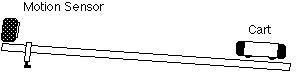
- Position the motion sensor at the high end of the track. The cart will
start at the low end of the track and be pushed up toward the motion sensor.
PART III: Preparing to Record Data
- Before recording any data for later analysis, you should experiment
with the motion sensor to make sure it is aligned and can "see"
the cart as it moves.
- Place the cart on the low end of the track (i.e., the end opposite
to the motion sensor)..
- Click the "REC" button to begin recording data.
- Give the cart a firm push up the track so the cart will move up the
inclined plane toward and then away from the motion sensor. BE CAREFUL!
Don't push the cart so firmly that it gets closer than 40 cm to the sensor.
- Click the "STOP" button to end recording your sample data
when the cart returns to the bottom of the track.
- Click the "Autoscale" button to automatically rescale the
Graph.
- If the plot of data is not smooth, check the alignment of the motion
sensor.
- Erase your sample run of data. Select "Run #1" in the Data
list in the Experiment Setup window...... and press the "Delete"
key.
PART IV: Data Recording
- Prepare to measure the motion of the cart as it moves toward the motion
sensor and then comes back down the track. Place the cart at the low end
of the track.
- Click the "REC" button to begin recording data. Give the
cart a firm push toward the motion sensor. Continue collecting data until
the cart has returned to the bottom of the track.
- Click the "STOP" button to end data recording.
- "Run #1" will appear in the Data list. (If the data points
do not appear on the graph, check the alignment of the motion sensor and
and try again.)
ANALYZING THE DATA
- Find the slope of the line of "best fit" in the plot of velocity
versus time. The slope is the average acceleration of the cart.
- Click the "Statistics" button in the lower left corner of the
Graph display to open the Statistics area in the right part of the Graph for
all three plots.
- Click the "Autoscale" button to rescale the graph to fit the data.
- In the plot of velocity, use the mouse to click-and-draw a rectangle around
the region of the plot that shows the cart's motion after the push and before
it stopped at the bottom of the track.
- Click the "Statistics Menu" button in the Statistics area of the
velocity plot. Select "Curve Fit, Linear Fit" from the Statistics
menu.
- The slope of the best fit line (coefficient "a2" in the
Statistics area) is the average acceleration. Record the value in the Data
Table.
- In the plot of acceleration, use the mouse to click-and-draw a rectangle
around the region of the plot that corresponds to the cart's motion after
the push and before it stopped at the bottom of the track.
- Click the Statistics menu button in the Statistics area. Select "Mean"
from the Statistics menu. The Statistics area of the acceleration plot
shows the mean value of the acceleration for your selected region.
- Record the mean of the acceleration.
- Calculate the theoretical value for the acceleration of the cart and record
it in the Data Table.

DATA TABLE
|
Height (m)
|
Angle (degrees)
|
Acceleration (slope) (m/s^2)
|
Acceleration (mean) (m/s^2)
|
Acceleration (theory) (m/s^2)
|
Difference (%)
|
|
|
|
|
|
|
|
|
|
|
|
|
|
|
|
|
|
|
|
|
|
|
|
|
|
|
|
|
|
|
|
|
|
|
|
|
|
|
|
|
|
|
|
|
|
|
|
|
|
|
|
|
|
|
|
|
|
|
|
|
|
|
|
QUESTIONS
- Describe the position versus time plot of the Graph display. Why does the
distance begin at a maximum and decrease as the cart moves up the inclined
plane?
- Describe the velocity versus time plot of the Graph display.
- Describe the acceleration versus time plot of the Graph display.
- How does the acceleration determined in the plot of velocity compare to
the mean value of acceleration from the plot of acceleration?
- What is the percent difference between the acceleration determined in the
plot of velocity and the theoretical value for acceleration? Remember:
© Frank L. H.
Wolfs, University of Rochester, Rochester, NY 14627, USA
Last updated on Sunday, February 11, 2001 22:42