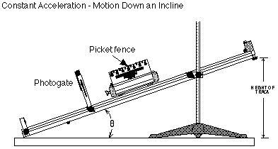
Constant Acceleration: Motion Down an Incline
Concept: linear motion
Time: 30 m
SW Interface: 700
Macintosh® file: P04 Constant Acceleration
Windows® file: P04_CONA.SWS
EQUIPMENT NEEDED
- Science Workshop Interface
- base and support rod
- photogate with mounting bracket
- five-pattern picket fence (for cart)
- dynamics cart
- meter stick
- track, 1.2 meter, with end-stop
PURPOSE
The purpose of this activity is to investigate how the acceleration of
an object down an incline depends on the angle of the incline and to obtain
the acceleration due to gravity.
THEORY
A cart on an incline will roll down the incline as it is pulled by gravity.
The direction of the acceleration due to gravity is straight down as shown
in the diagram. The component of the acceleration due to gravity which is
parallel to the inclined surface is gsin ø where ø is the
angle of the incline. Neglecting friction, this is the acceleration of the
cart.
PROCEDURE
In this activity you will use a photogate to measure the motion of a
cart as it moves down an inclined track. To find the acceleration of the
cart, the cart will be started from rest and a "picket fence"
mounted on the cart will pass through the photogate beam. The acceleration
of the cart will be calculated from the derivative of the velocity. The
sine of the angle (sin ø) will be calculated from the height of the
track and the length of the track.

The slope of a graph of the cart's acceleration versus sin ø gives
the value of "g", the acceleration due to gravity.
* NOTE: This activity is easier to do if you have a partner to run the
computer while you release the cart.
PART I: Computer Setup
- Connect the Science Workshop interface to the computer, turn
on the interface, and turn on the computer.
- Connect the photogate's stereo phone plug to Digital Channel 1 on the
interface.
- Open the Science Workshop file titled as shown:
- Macintosh: P04 Constant Acceleration
- Windows: P04_CONA.SWS
The document has a Graph display. The vertical axis of the Graph shows
"Acceleration (m/sec/sec)", which is a calculation based on the
derivative of velocity. The horizontal axis shows "sin ø",
which is a calculation based on the height of the raised end of the track,
and the overall length of the track (hypotenuse). (Note: For quick reference,
see the Experiment Notes window. To bring a display to the top, click on
its window or select the name of the display from the list at the end of
the Display menu. Change the Experiment Setup window by clicking on the
"Zoom" box or the Restore button in the upper right hand corner
of that window.)
- The "Sampling Options..." for this experiment are as follows:
Periodic Samples = Fast at 10 Hz, Digital Timing = 10000 Hz.
- The Science Workshop program calculates the velocity of the
cart based on the distance between the leading edges of the opaque bands
of the picket fence. The top row of the "five pattern picket fence"
has opaque bands that are 1 centimeter from leading edge to leading edge.
This value for the distance has been entered in the setup window for the
"Photogate & Picket Fence".
- If you are using a picket fence with a different distance between the
leading edges of the opaque bands, change the value in the setup window
for the sensor (as follows).
- Double-click the Photogate & Picket Fence icon in the Experiment
Setup window to open the sensor setup window.
- Enter the correct distance for "Opaque Band Spacing" in the
sensor setup window. Click "OK" to return to the Experiment Setup
window.
- The Science Workshop program calculates the value of sin ø
by dividing the height of the raised end of the track by the overall length
of the track. The PASCO scientific dynamics track is 1.22 meters
or 122 centimeters long. This value for the overall length has been entered
in the Experiment Calculator. However, it is important to enter the length
of your track.
- Carefully measure the overall length of your track and change the value
in the Experiment Calculator.
- Click the Calculator button in the Experiment Setup window to open
the Experiment Calculator window.
- The formula in the Experiment Calculator shows "@K/122".
The first part (@K) represents the Keyboard entered values for the height
of the track. The second part (122) is the length of the track in centimeters.
- Highlight the part of the formula that represents the length of the
track. Enter your measured value for the track. Click the "equals"
button in the keypad, or press <return> or <enter> on the keyboard
to record your changed value.
- You can close the Experiment Calculator by clicking the "close"
box or by double-clicking the "control-menu" box in the upper
left corner of the window.
PART II: Sensor Calibration and Equipment Setup
- You do not need to calibrate the photogate for this activity.
- Level the track by setting the cart on the track to see which way it
rolls. Adjust the leveling screw at the end of the track to raise or lower
that end until the cart placed at rest on the track will not move toward
either end. Record the height of the end of the track that does not have
the end-stop.
- Put the picket fence in the slots on the top of the dynamics cart with
the 1 centimeter row on top. Attach the photogate with mounting bracket
to the track. Position the photogate so the cart will have room to begin
to move before the picket fence passes through it. Adjust the photogate
height so the 1 centimeter row of the picket fence will pass through the
photogate beam.
- Set up the track as shown in the diagram, raising the end of the track
without an end-stop so that it is 10 cm higher than its position when level.
- Use a pencil to put a mark near the midpoint of the track.
- Let the midpoint mark be your starting point for the cart release during
data recording.

Preparing to Record Data
- Before recording any data for later analysis, you should experiment
with the photogate, cart, and picket fence. Put the cart at the starting
point on the track
- Click the "REC" button in the Experiment Setup window. The
"Keyboard Sampling" window opens.
- Put the cart at the starting point on the track. Release the cart so
it moves down the track.
- After the cart moves through the photogate, type in the height of the
raised end of the track as "Entry #1". For this example, the
default value is already "10.0000", (10 centimeters or 0.10 meters).
Click "Enter".
- Click "Stop Sampling" to end recording of your sample data.
"Run #1" will appear in the Experiment Setup window.
- Click the "Autoscale" button in the Graph display.
- Erase your trial run of data. Select "Run #1" in the
Data list in the Experiment Setup window ...... and press the "Delete"
key.
PART III: Data Recording
- Click the "REC" button to begin data recording. The "Keyboard
Sampling" window opens. Move the window so you can see it throughout
the experiment.
- Put the cart at the starting point on the track. Release the cart so
it moves through the photogate.
- After the cart moves through the photogate, type in the height of the
raised end of the track as "Entry #1" in the Keyboard Sampling
window. Click the "Enter" button to record your value for the
height of the track. (NOTE: The default value in the Keyboard Sampling
window is "10.0000", so you do not need to type in a value for
the first entry.)
- The Keyboard Sampling window will display your entered value in the
Data list.
- Lower the raised end of the track by one centimeter.
- Repeat the procedure at the new height. Put the cart at the starting
point on the track. Release the cart. After the cart moves through the
photogate, type in the new height as "Entry #2".
- Click "Enter" to record your new value for the height of
the track.
- NOTE: The default value for Entry #3 in the Keyboard Sampling window
reflects the pattern of the your first two recorded values.
- Continue to repeat the procedure. Lower the raised end of the track
by one centimeter each time until the raised end is at 4 centimeters.
- Click the "STOP" button to end data recording.
- "Run #1" will appear in the Data list in the Experiment Setup
window.
ANALYZING THE DATA
- Click the "Statistics" button in the lower left corner of
the Graph to open the Statistics area. Click the "Autoscale"
button to automatically rescale the Graph to fit the data.
- In the Statistics area, click the "Statistics Menu" button
. Select "Curve Fit, Linear Fit" from the Statistics menu.
- The value of coefficient "a2" in the Statistics area is the
slope of the best fit line for the data. Record this value as the acceleration
due to gravity, "g".
acceleration due to gravity, "g" = _________
m/s/s
QUESTIONS
- What is the percent difference between your measured value for "g"
and the accepted value for "g"?
- Remember,

- If the mass of the cart is doubled, how are the results affected ?
Try it.
© Frank L. H.
Wolfs, University of Rochester, Rochester, NY 14627, USA
Last updated on Sunday, February 11, 2001 21:24
![]()
