Understanding Motion I: Distance and Time
Concept: linear motion
Time: 30 m
SW Interface: 700
Macintosh® file: P01 Understanding Motion 1
Windows® file: P01_MOT1.SWS
EQUIPMENT NEEDED
- Science Workshop Interface
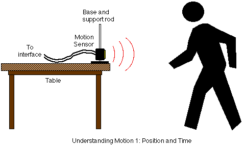
- Base and support rod
- Motion sensor
PURPOSE
The purpose of this activity is to introduce the relationships between
the motion of an object - YOU - and a Graph of position and time for the
moving object.
NOTE: This activity is easier to do if you have a partner to run the
computer while you move.
THEORY
When describing the motion of an object, knowing where it is relative
to a reference point, how fast and in what direction it is moving, and how
it is accelerating (changing its rate of motion) is essential. A sonar ranging
device such as the Motion Sensor uses pulses of ultrasound that reflect
from an object to determine the position of the object. As the object moves,
the change in its position is measured many times each second. The change
in position from moment to moment is expressed as a velocity (meters per
second). The change in velocity from moment to moment is expressed as an
acceleration (meters per second per second). The position of an object at
a particular time can be plotted on a graph. You can also graph the velocity
and acceleration of the object versus time. A graph is a mathematical picture
of the motion of an object. For this reason, it is important to understand
how to interpret a graph of position, velocity, or acceleration versus time.
In this activity you will plot a graph in real-time, that is, as the motion
is happening.
PROCEDURE
For this activity, you will be the object in motion. The Motion Sensor will
measure your position as you move in a straight line at different speeds. The
Science Workshop program will plot your motion on a graph of position and time.
The challenge in this activity is to move in such a way that a plot of your
motion on the same graph will "match" the line that is already there.
PART I: Computer Setup
- Connect the Science Workshop interface to the computer, turn on the interface,
and turn on the computer.
- Connect the motion sensor's stereo phone plugs to Digital Channels 1 and
2 on the interface. Connect the yellow-taped plug to Digital Channel 1 and
the other plug to Digital Channel 2.
- Goto the "/Global Shared f/PHY105 Tools/Experiments/" shared folder
and click on the "Playing with the motion sensor" button. This will
open Scientific Workshop and load the experimental setup.
- The "Sampling Options..." for this experiment are as follows:
Periodic Samples = Fast at 10 Hz, Digital Timing = 10000 Hz, and Stop Condition
with Time = 10.00 seconds.
PART II: Sensor Calibration and Equipment Setup
- Mount the motion sensor on a support rod so that it is aimed at your
midsection when you are standing in front of the sensor. Make sure that
you can move at least 2 meters away from the motion sensor.
NOTE: You will be moving backwards for part of this activity. Clear
the area behind you for at least 2 meters (about 6 feet).
- Position the computer monitor so you can see the screen while you move
away from the motion sensor.
- Stand in front of the motion sensor and hit the record button. You
will hear the sound being emitted by the motion sensor. It is the reflection
of this sound that is being used by the sensor to determine the distance
between the sensor and you.
- Move back and forth in front of the sensor and see how the measured
position changes.
- Use a ruler to make measurements at some well-defined distances. Compare
the values obtained by the motion sensor with the directly measured values.
- Do they agree?
- Are they always exaclty the same?
- Is the motion sensor calibrated correctly?
- Select open from the file menu and select "P00a Motion sensor"
from the "/Global Shared f/PHY105 Tools/Experiments/" shared
folder. What is the maximum and the minimum range of the motion sensor.
- Repeat the previous measurements using the "P00b Motion sensor"
and "P00c Motion sensor" setups. Can you explain the observed
differences?
PART III: Data Recording
- Save your data in your own folder
- Open "P01 Understanding Motion 1" in the "/Global Shared
f/PHY105 Tools/Experiments/" shared folder . This will open the Scientific
Workshop and load the experimental setup.
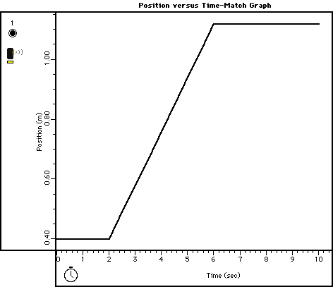
- The document shows the following Graph display of Position (m) and Time
(sec).
- (Note: For quick reference, see the Experiment Notes window. To bring
a display to the top, click on its window or select the name of the display
from the list at the end of the Display menu. Change the Experiment Setup
window by clicking on the "Zoom" box or the Restore button in
the upper right hand corner of that window.)
- Click on the Graph to make it active. Enlarge the Graph until it fills the
monitor screen.
- Study the Position versus Time plot in order to determine the following:
- How close should you be to the motion sensor at the beginning? _______
(m)
- How far away should you move? _______ (m)
- How long should your motion last? _______ (sec)
- When you are ready, stand in front of the motion sensor. WARNING: You
will be moving backward, so be certain that the area behind you is free of
obstacles.
- Click the "REC" button to begin recording data. (Data recording
will begin almost immediately. The motion sensor will make a faint clicking
noise.)
- Watch the plot of your motion on the Graph, and try to move so that the
plot of your motion matches the Position vs Time plot that is already there.
- Data recording will end automatically after a certain amount of time, or
click on "STOP" to end sooner. Run #1 will appear in the Data list
in the Experiment Setup window.
- Repeat the data recording process a second and a third time. Try to improve
the match between the plot of your motion and the plot that is already on
the Graph.
OPTIONAL
The Graph can show more than one run of data at the same time. You can display
up to three runs simultaneously. If you record more than three runs, use the
DATA menu along the vertical axis to select the runs you want to see. To delete
a run of data, click on the run in the Data list in the Experiment Setup window
and press the "delete" key on the keyboard.
ANALYZING THE DATA
- Use the Statistics tools in the Graph to determine the slope of the best
fit line for the middle section of your best position vs. time plot. Click
the "Statistics" button and then click the "Autoscale"
button to resize the graph to fit the data.
- Use the mouse to click-and-draw a rectangle around the middle section of
your plot. Use the "Statistics" menu button in the Statistics area
of the Graph. Select "Linear Fit" from the Curve Fit menu to display
the slope of the selected region of your position vs time plot. The "a2"
term of the equation in the Stats area is the slope of the selected region
of motion. The slope of this part of the position vs. time plot is the velocity
during the selected region of motion.
- Determine how well your plot of motion fits the plot that was already in
the Graph. Examine the "total abs. difference" (total absolute difference)
and the chi^2 (goodness of fit) terms from the Statistics area.
QUESTIONS
- In the Graph, what is the slope of the line of best fit for the middle
section of your plot?
- What is the description of your motion? (Example: "Constant speed
for 2 seconds followed by no motion for 3 seconds, etc.")
© Frank L. H.
Wolfs, University of Rochester, Rochester, NY 14627, USA
Last updated on Monday, January 22, 2001 8:16