NOTE
This manual describes the laboratory experiment used during the 1996 - 1997 academic year. Significant changes have been made since then, and the manual used during the current academic year is in NOT available yet on the WEB. Hardcopies can be purchased at the bookstore.
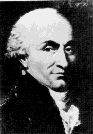
Charles Augustin de Coulomb
(koolom) 1736-1806
To verify the proportionality of Coulomb's Law that the electric force between two point charges is directly proportional to the product of the charges and is inversely proportional to the square of the distance between them.
Coulomb's Law gives us the static electrical force F, exerted by a point charge Q1 on another point charge Q2 in terms of r, the distance between them :
F = Q1 Q2 / 40 r2 ( 6.1)
In this experiment, we will verify this law and also learn how to use an optical lever to magnify a small rotation into a large displacement. Finally we will learn about systematic errors and how to correct for them.
The prelab homework must be handed to the lab TA before you start the lab.
1. The electric force depends on the distance r, in a certain way. Can you think of another force in nature which also obeys an " inverse - square" law ?
2. Consider the function y = xn (for n = -2 ). Take the natural logarithm of both sides and plot ln y vs. ln x on linear - linear paper. Show how to obtain "n".
The verification of Coulomb's Law proceeds as follows :
1. Charges are put on the spherical conductors.
2. Because of the charge there is a force between the two spheres.
3. The force (F) between the spheres will produce a deflection ( ) of the sphere attached to the torsion fiber. These two quantities are related
F = k ( 6.2 )
where k is the torsion constant of the fiber.
4. The Q dependence is measured by adding charge ( to Q1 , say ) , keeping r constant and measuring ( and inferring F ).
5. The separation dependence is measured by charging the spheres and measuring ( and inferring F ) for various separations r.
The actual experiment will be executed as follows :
1. Clean the spheres and insulators with alcohol ; dry them with tissue paper and drier. This ensures that no charges apart from the ones we place on the spheres influence the experiment.
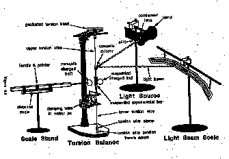
2. The optical lever system for measuring must be adjusted. Adjust the torsion head so that the wire is taut and the damping vane is at the center of the beaker so that it can move without being obstructed by the glass walls.
3. Adjust the lamp and place the stand of the scale 1.2m away from the mirror to get a sharp image about 25cm from the right end (looking from the mirror) of the circular scale, on which each graduation is 1 cm. make sure that the image does not go off the scale for maximum deflection 0 of the light beam.The light source, the mirror and the scale should all be in a horizontal plane.
Although we are interested in the static deflection of the optical lever system to infer the force F, we have to acknowledge that this system is a torsion oscillator and the transient behavior to static changes must be determined. There is an oscillatory period t0 and a damping or relaxation time tr .The angular displacement due to these transients is given by :
( t ) = 0 exp ( - t / tr ) cos ( 2 t / t0 ) (6.3)
from where we can see that at time t = t r
( t ) = 0 exp ( -1 ) 0 / 3
(Here we have used the fact that for critical damping, t0 ~ tr ). So the reason we wait till the displacement becomes a third of the original 0 is that the time interval t then equals tr. tr is called the " relaxation time" and is the approximate time that the torsion oscillator takes to settle down to its equilibrium value. Actually 1/3 is here an approximation for the number 1/e = 1/ 2.71... and is therefore not fundamental and is only an approximation. Each time we vary the charge or the distance, we should wait ~ 3tr seconds before taking down a reading:
1. Touch the spheres with the grounding probe - this makes them totally neutral.
2. Perturb the optical lever system by blowing on the sphere attached to the torsion. Obtain about 15-20cm displacement (0). Note 0 , and start the timer.Stop when displacement ( ) = 0 /3. The time measured will then equal tr.
Because of air currents and humidity, charge tends to leak off from the spheres. The leakage is not negligible and has to be accounted for. This will enable you to make a correction to the charge in your later measurements.
1. Adjust the movable sphere such that the pointer on the scale reads 3.0 cm ; bring the movable sphere and stand as near as you can to the sphere on the torsion without making them touch. Since the radius of each sphere is 1.5cm the distance between their centers ( 3cm ) can now be directly read off the scale ( 3cm ! ). The heights of the spheres from the table should be equal. The stand should not be moved for the rest of the experiment.
2. Rub the lucite rod with silk. " Scrape" ( your TA will demonstrate this) across the sphere attached to the torsion to transfer charge. This will introduce an opposite " image" charge on the sphere attached to the fiber. It will move towards the movable sphere attached to the scale, finally touching it. Once the spheres touch, the charges will be equally distributed between them and since they now will have the same charge, they will begin to repel each other. The sphere on the torsion fiber will now begin to move away from the movable sphere, and the light image will register a deflection on the circular scale. You should keep increasing the charge till = 0 25cm ( This is not critical ; 20 or 32 cm will work just as well). Start the timer.
3. Note the decrease of as time elapses ; that is, record vs. t every centimeter as = 25,24,23, ...0 cm. The leakage of charge might turn out to be an exponential decay, i.e. the displacement at any time t would be given by :
( t ) = 0 exp ( - t / td ) ( 6.3 )
where 0 is the initial displacement and the decay is characterized by a " time constant" td. To find td we wait for the displacement to become a third of initial value just as we did for tr.
4. Plot a normalized deflection ln [ / 0 ] vs. t "decay curve" on linear graph paper. If the deflection is exponential, you should observe a straight line. Whatever curve you measure will be used to correct for leakage in later readings of in the Q1 and r sections (Parts IV and V below ) by reading off the fraction of charge that has been lost ( the amount by which the displacement has resultantly decreased ) and adding it to whatever you have measured.
Now we will actually begin making measurements to test Coulomb's Law. In this section we vary the charge .
1. Ground spheres ; obtain equilibrium.
2. Set sphere on scale to 3.5 cm. Charge spheres to get 20-30cm deflection.
3. Set sphere on scale to 5cm.Start timer ; note , after the transient dies out. (Do not stop the timer.)
Note : If we set r = 5cm before charging , the amount of charge we will have to put on the spheres to get a 20-30cm deflection is going to be rather large - remember that the electric force F ( here ) is proportional to 1 / r2 , i.e., it weakens rapidly with distance. If we still keep r = 3.5cm after charging , we might find ourselves in the regime where there are complications due to the image charges that the spheres induce in each other. Hence we start taking readings with r = 5cm.
4. Ground test sphere ; touch it to the movable sphere, thus halving its charge. Record , t when the displacement stabilizes.
5. Here we used the fact that the uncharged test sphere, when brought into contact with the sphere on the torsion fiber ( carrying charge Q1 ) will take away half its charge, leaving it with Q1 /2. To vary Q1 further, we will ground the test charge and touch it to Q1 /2, halving it to Q1 /4 and then record the corresponding , t.
6. Repeat the halving procedure until you reach Q1 /8 or the deflection is too small to measure.
The procedure is similar to that of Part IV above.
1. Ground spheres ; obtain equilibrium.
2. Set the movable sphere to 3.5 cm. Charge spheres to get 20 - 30 cm deflection.
3. Set the movable sphere to 5 cm to make the image charge effects small. start timer; note , t after the transients have died down. Do not stop the timer.
4. Set the sphere on the scale to 10, 15, and 20 cm ; record , t after each change of scale.
Due to possible changes in humidity and other conditions of the air we measure the decay curve and plot it on the same graph as Part III above.
1. Compare the before and after plots of normalized deflection ln [ /0 ] vs. time t. If they are different use their average - which is NOT just a line half - way between the two - as the correction for the corresponding - values. The difference between the average and the two curves will be the error (i.e. the error bars will touch both the plotted lines ).
2. Plot the deflection ( decay-corrected ) vs. charge data taken in part IV above on linear graph paper.
3. Plot the ln [ deflection ( decay - corrected ) ] vs. separation data taken in part V above on linear paper. Here you may wish to neglect the points for small separations where the image charge effects are the largest and the graph might deviate from a straight line. Draw a best - fitting straight line. What is the slope of this line ? Do the results indicate a " power law" ? If so, what is your best estimate of the exponent ?