Chapter 5. Magnetostatics
5.1. The Magnetic Field
Consider two parallel straight wires in which current is flowing. The
wires are neutral and therefore there is no net electric force between the
wires. Nevertheless, if the current in both wires is flowing in the same
direction, the wires are found to attract each other. If the current in one of
the wires is reversed, the wires are found to repel each other. The force
responsible for the attraction and repulsion is called the magnetic
force. The magnetic force acting on a moving charge q is defined in
terms of the magnetic field:
The vector product is required since observations show that the force
acting on a moving charge is perpendicular to the direction of the moving
charge. In a region where there is an electric field and a magnetic field the
total force on the moving force is equal to
This equation is called the Lorentz force law and provides us with
the total electromagnetic force acting on q. An important difference
between the electric field and the magnetic field is that the electric field
does work on a charged particle (it produces acceleration or deceleration) while
the magnetic field does not do any work on the moving charge. This is a direct
consequence of the Lorentz force law:

We conclude that the magnetic force can alter the direction in which a
particle moves, but can not change its velocity.
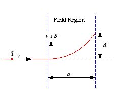
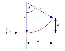
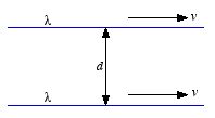
Example: Problem
5.1 A particle of charge
q enters the region of uniform magnetic
field

(pointing into the page). The field deflects the particle a distance
d
above the original line of flight, as shown in Figure 5.1. Is the charge
positive or negative? In terms of
a,
d,
B, and
q,
find the momentum of the particle.
In order to produce the observed
deflection, the force on
q at the entrance of the field region must be
directed upwards (see Figure 5.1). Since direction of motion of the particle
and the direction of the magnetic field are known, the Lorentz force law can be
used to determine the direction of the magnetic force acting on a positive
charge and on a negative charge. The vector product between

and
points upwards in Figure 5.1 (use the right-hand rule). This shows that the
charge of the particle is positive.
 Figure
1. Problem 5.1.
Figure
1. Problem 5.1.The magnitude of the force acting on the moving charge is equal
to
As a result of the magnetic force, the charged particle will follow a
spherical trajectory. The radius of the trajectory is determined by the
requirement that the magnetic force provides the centripetal force:
In this equation r is the radius of the circle that describes the
circular part of the trajectory of charge q. The equation can be used to
calculate r:
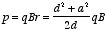
where p is the momentum of the particle. Figure 5.2 shows the
following relation between r, d and a:
This equation can be used to express r in terms of d and
a:
The momentum of the charge q is therefore equal to
 Figure
2. Problem 5.2.
Figure
2. Problem 5.2. The electric current in a wire is due to the motion of the electrons in the
wire. The direction of current is defined to be the direction in which the
positive charges move. Therefore, in a conductor the current is directed
opposite to the direction of the electrons. The magnitude of the current is
defined as the total charge per unit time passing a given point of the wire
(I = dq/dt). If the current flows in a region with a non-zero
magnetic field then each electron will experience a magnetic force. Consider a
tiny segment of the wire of length dl. Assume that the electron density
is -λ C/m and that each electron is moving with a velocity
v. The magnetic force exerted by the magnetic field on a single electron
is equal to
A segment of the wire of length dl contains λ dl/e
electrons. Therefore the magnetic force acting in this segment is equal
to
Here we have used the definition of the current I in terms of
dq and dt:
In this derivation we have defined the direction of

to be equal to the direction of the current (and therefore opposite to the
direction of the velocity of the electrons). The total force on the wire is
therefore equal to
Here I have assumed that the current is constant throughout the wire. If
the current is flowing over a surface, it is usually described by a
surface
current density

,
which is the current per unit length-perpendicular-to-flow. The force on a
surface current is equal to
If the current flows through a volume, is it is usually described in terms
of a
volume current density

.
The magnetic force on a volume current is equal to
The surface integral of the current density
across the surface of a volume
V is equal to the total charge leaving the
volume per unit time (charge conservation):
Using the divergence theorem we can rewrite this expression as
Since this must hold for any volume V we must require that
This equation is known as the continuity equation.
5.2. The Biot-Savart Law
In this Section we will discuss the magnetic field produced by a steady
current. A steady current is a flow of charge that has been going on
forever, and will be going on forever. These currents produce magnetic fields
that are constant in time. The magnetic field produced by a steady line current
is given by the Biot-Savart Law:
where
is an element of the wire,

is the vector connecting the element of the wire and
P, and

is the permeability constant which is equal to
The unit of the magnetic field is the Tesla (T). For surface
and volume currents the Biot-Savart law can be rewritten as
and
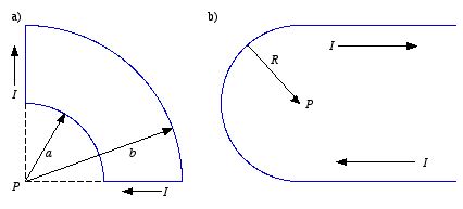
Example: Problem 5.9 Find the magnetic field at point
P for each of the steady current configurations shown in Figure
5.3.
a) The total magnetic field at
P is the vector sum of the
magnetic fields produced by the four segments of the current loop. Along the
two straight sections of the loop,

and
are parallel or opposite, and thus

.
Therefore, the magnetic field produced by these two straight segments is equal
to zero. Along the two circular segments
and
are perpendicular. Using the right-hand rule it is easy to show that
and
where

is pointing out of the paper. The total magnetic field at
P is therefore
equal to
 Figure
5.3. Problem 5.9.
Figure
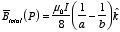
5.3. Problem 5.9.b) The magnetic field at P produced by the circular segment of the
current loop is equal to
where
is pointing out of the paper. The magnetic field produced at
P by each
of the two linear segments will also be directed along the negative
z
axis. The magnitude of the magnetic field produced by each linear segment is
just half of the field produced by an infinitely long straight wire (see Example
5 in Griffiths):
The total field at P is therefore equal to
Example: Problem 5.12
Suppose you have two infinite
straight-line charges λ, a distance d apart, moving along at
a constant v (see Figure 5.4). How fast would v have to be in
order for the magnetic attraction to balance the electrical repulsion?
 Figure
5.4. Problem 5.12.
Figure
5.4. Problem 5.12. When a line charge moves it looks like a current of magnitude I =
λv. The two parallel currents attract each other, and the
attractive force per unit length is
and is attractive. The electric generated by one of the wires can be found
using Gauss' law and is equal to
The electric force per unit length acting on the other wire is equal
to
and is repulsive (like charges). The electric and magnetic forces are
balanced when
or
This requires that
This requires that the speed v is equal to the speed of light, and
this can therefore never be achieved. Therefore, at all velocities the electric
force will dominate.
5.3. The Divergence and Curl of B.
Using the Biot-Savart law for a volume current

we can calculate the divergence and curl of

:
and
This last equation is called Ampere's law in differential form.
This equation can be rewritten, using Stokes' law, as
This equation is called
Ampere's law in integral form. The
direction of evaluation of the line integral and the direction of the surface
element vector

must be consistent with the right-hand rule.
Ampere's law is always true,
but is only a useful tool to evaluate the magnetic field if the symmetry of the
system enables you to pull

outside the line integral. The configurations that can be handled by Ampere's
law are:
1. Infinite straight lines
2. Infinite planes
3. Infinite
solenoids
4. Toroids
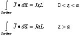
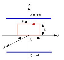
Example: Problem 5.14 A thick slab
extending from
z = -
a to
z =
a carries a uniform
volume current

.
Find the magnetic field both inside and outside the slab.
 Figure
5.5. Problem 5.14
Figure
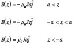
5.5. Problem 5.14 Because of the symmetry of the problem the magnetic field will be directed
parallel to the
y axis. The magnetic field in the region above the
xy plane (
z > 0) will be the mirror image of the field in the
region below the
xy plane (
z < 0). The magnetic field in the
xy plane (
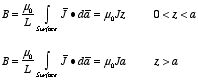
z = 0) will be equal to zero. Consider the Amperian
loop shown in Figure 5.5. The current is flowing out of the paper, and we
choice the direction of
to be parallel to the direction of

.
Therefore,
The direction of evaluation of the line integral of

must be consistent with our choice of the direction of
(right-hand rule). This requires that the line integral of
must be evaluated in a counter-clockwise direction. The line integral of
is equal to
Applying Ampere's law we obtain for
:
Thus
5.4. The Vector Potential
The magnetic field generated by a static current distribution is uniquely
defined by the so-called Maxwell equations for magnetostatics:
Similarly, the electric field generated by a static charge distribution is
uniquely defined by the so-called Maxwell equations for
electrostatics:
The fact that the divergence of
is equal to zero suggests that there are no point charges for
.
Magnetic field lines therefore do not begin or end anywhere (in contrast to
electric field lines that start on positive point charges and end on negative
point charges). Since a magnetic field is created by moving charges, a magnetic
field can never be present without an electric field being present. In
contrast, only an electric field will exist if the charges do not
move.
Maxwell's equations for magnetostatics show that if the current
density is known, both the divergence and the curl of the magnetic field are
known. The Helmholtz theorem indicates that in that case there is a
vector
potential

such that
However, the vector potential is not uniquely defined. We can add to it
the gradient of any scalar function f without changing its
curl:
The divergence of

is equal to
It turns out that we can always find a scalar function
f such that
the vector potential
is divergence-less. The main reason for imposing the requirement that

is that it simplifies many equations involving the vector potential. For
example, Ampere's law rewritten in terms of
is
or
This equation is similar to Poisson's equation for a charge distribution
ρ:
Therefore, the vector potential
can be calculated from the current

in a manner similar to how we obtained
V from
ρ.
Thus
Note: these solutions require that the currents go to zero at
infinity (similar to the requirement that
ρ goes to zero at
infinity).
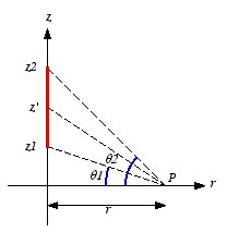
Example: Problem 5.22 Find the magnetic vector
potential of a finite segment of straight wire carrying a current
I.
Check that your answer is consistent with eq. (5.35) of Griffiths.
The
current at infinity is zero in this problem, and therefore we can use the
expression for

in terms of the line integral of the current
I. Consider the wire
located along the
z axis between
z1 and
z2 (see Figure 5.6) and use cylindrical coordinates. The
vector potential at a point
P is independent of
φ
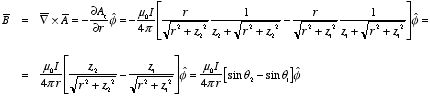
(cylindrical symmetry) and equal to
Here we have assumed that the origin of the coordinate system is chosen
such that P has z = 0. The magnetic field at P can be
obtained from the vector potential and is equal to
where θ1 and θ2 are defined
in Figure 5.6. This result is identical to the result of Example 5 in
Griffiths.
 Figure
5.6. Problem 5.25.
Figure
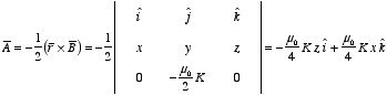
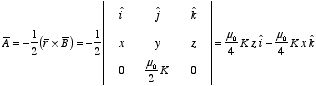
5.6. Problem 5.25. Example: Problem 5.24 If

is
uniform, show that

,
where

is the vector from the origin to the point in question. That is check that

and

.
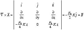
The
curl of
is equal to
Since
is uniform it is independent of
r,
θ, and
φ and
therefore the second and third term on the right-hand side of this equation are
zero. The first term, expressed in Cartesian coordinates, is equal to
The fourth term, expressed in Cartesian coordinates, is equal to
Therefore, the curl of

is equal to
The divergence of
is equal to
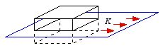
Example: Problem 5.26
Find the vector potential above and
below the plane surface current of Example 5.8 in Griffiths.
In Example
5.8 of Griffiths a uniform surface current is flowing in the xy plane,
directed parallel to the x axis:
However, since the surface current extends to infinity, we can not use the
surface integral of

to calculate

and an alternative method must be used to obtain
.
Since Example 8 showed that

is uniform above the plane of the surface current and
is uniform below the plane of the surface current, we can use the result of
Problem 5.27 to calculate
:
In the region above the xy plane (z > 0) the magnetic
field is equal to
Therefore,
In the region below the xy plane (z < 0) the magnetic
field is equal to
Therefore,
We can verify that our solution for
is correct by calculating the curl of
(which must be equal to the magnetic field). For
z > 0:
The vector potential
is however not uniquely defined. For example,

and

are also possible solutions that generate the same magnetic field. These
solutions also satisfy the requirement that
.
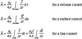
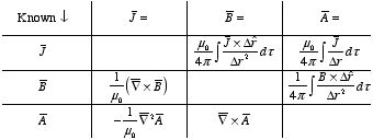
5.5. The Three Fundamental Quantities of
Magnetostatics
Our discussion of the magnetic fields produced by steady currents has
shown that there are three fundamental quantities of magnetostatics:
1. The
current density

2. The
magnetic field

3. The
vector potential
These
three quantities are related and if one of them is known, the other two can be
calculated. The following table summarizes the relations between
,
,
and
:
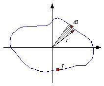
5.6. The Boundary Conditions of B
In Chapter 2 we studied the boundary conditions of the electric field and
concluded that the electric field suffers a discontinuity at a surface charge.
Similarly, the magnetic field suffers a discontinuity at a surface
current.
 Figure
5.7. Boundary conditions for
.
Figure
5.7. Boundary conditions for
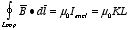
. Consider the surface current

(see Figure 5.7). The surface integral of
over a wafer thin pillbox is equal to
where
A is the area of the top and bottom of the pill box. The
surface integral of
can be rewritten using the divergence theorem:
since
for any magnetic field
.
Therefore, the perpendicular component of the magnetic field is continuous at a
surface current:
The line integral of
around the loop shown in Figure 5.8 (in the limit
ε → 0) is
equal to
According to Ampere's law the line integral of
around this loop is equal to
 Figure
5.8. Boundary conditions for
.
Figure
5.8. Boundary conditions for
.Therefore, the boundary condition for the component of
,
parallel to the surface and perpendicular to the current, is equal to
The boundary conditions for
can be combined into one equation:
where

is a unit vector perpendicular to the surface and the surface current and
pointing "upward". The vector potential

is continuous at a surface current, but its normal derivative is not:
5.7. The Multipole Expansion of the Magnetic
Field
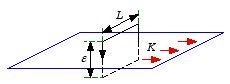
To calculate the vector potential of a localized current distribution at
large distances we can use the multipole expansion. Consider a current loop
with current I. The vector potential of this current loop can be written
as
At large distance only the first couple of terms of the multipole expansion
need to be considered:
The first term is called the
monopole term and is equal to zero
(since the line integral of

is equal to zero for any closed loop). The second term, called the
dipole
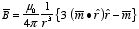
term, is usually the dominant term. The vector potential generated by the
dipole terms is equal to
This equation can be rewritten as
where

is called the
magnetic dipole moment of the current loop. It is defined
as
If the current loop is a plane loop (current located on the surface of a
plane) then

is the area of the triangle shown in Figure 5.9. Therefore,
where a is the area enclosed by the current loop. In this case, the
dipole moment of the current loop is equal to
where the direction of

must be consistent with the direction of the current in the loop (right-hand
rule).
 Figure
5.9. Calculation of
.
Figure
5.9. Calculation of
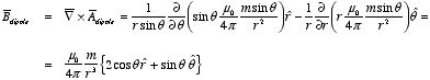
. Assuming that the magnetic dipole is located at the origin of our
coordinate system and that
is pointing along the positive
z axis, we obtain for

:
The corresponding magnetic field is equal to
The shape of the field generated by a magnetic dipole is identical to the
shape of the field generated by an electric dipole.
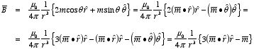
Example: Problem
5.33
Show that the magnetic field of a dipole can be written in the
following coordinate free form:
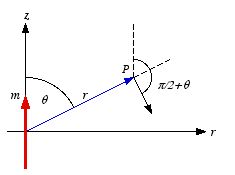 Figure
5.10. Problem 5.33.
Figure
5.10. Problem 5.33. Consider the configuration shown in Figure 5.10. The scalar product
between

and

is equal to
The scalar product between

and
is equal to
Therefore,
Example: Problem 5.34
A circular loop of wire, with radius
R, lies in the xy plane, centered at the origin, and carries a
current I running counterclockwise as viewed from the positive z
axis.
a) What is its magnetic dipole moment?
b) What is its (approximate)
magnetic field at points far from the origin?
c) Show that, for points on the
z axis, your answer is consistent with the exact field as calculated in
Example 6 of Griffiths.
a) Since the current loop is a plane loop, its
dipole moment is easy to calculate. It is equal to
b) The magnetic field at large distances is approximately equal
to
c) For points on the positive z axis θ = 0°.
Therefore, for z>0
Fore points on the negative z axis θ = 180°.
Therefore, for z<0
The exact solution for

on the positive
z axis is
For z » R the field is approximately equal to
which is consistent with the dipole field of the current
loop.
Example: Problem 5.35
A phonograph record of radius
R, carrying a uniform surface charge σ, is rotating at
constant angular velocity ω. Find its magnetic dipole
moment.
The rotational period of the disk is equal to
Consider the disk to consist of a large number of thin rings. Consider a
single ring of inner radius r and with dr. The charge on such a
ring is equal to
Since the charge is rotating, the moving charge corresponds to a current
dI:
The dipole moment of this ring is therefore equal to
The total dipole moment of the disk is equal to