Chapter 3. Special Techniques for Calculating
Potentials
Given a stationary charge distribution

we can, in principle, calculate the electric field:
where

.
This integral involves a vector as an integrand and is, in general, difficult to
calculate. In most cases it is easier to evaluate first the electrostatic
potential
V which is defined as
since the integrand of the integral is a scalar. The corresponding
electric field

can then be obtained from the gradient of
V since
The electrostatic potential V can only be evaluated analytically for
the simplest charge configurations. In addition, in many electrostatic
problems, conductors are involved and the charge distribution ρ is
not known in advance (only the total charge on each conductor is known).
A
better approach to determine the electrostatic potential is to start with
Poisson's equation
Very often we only want to determine the potential in a region where
ρ = 0. In this region Poisson's equation reduces to Laplace's
equation
There are an infinite number of functions that satisfy Laplace's equation
and the appropriate solution is selected by specifying the appropriate
boundary conditions. This Chapter will concentrate on the various
techniques that can be used to calculate the solutions of Laplace's equation and
on the boundary conditions required to uniquely determine a
solution.
3.1. Solutions of Laplace's Equation in One-, Two, and Three
Dimensions
3.1.1. Laplace's Equation in One Dimension
In one dimension the electrostatic potential V depends on only one
variable x. The electrostatic potential V(x) is a solution
of the one-dimensional Laplace equation
The general solution of this equation is
where s and b are arbitrary constants. These constants are
fixed when the value of the potential is specified at two different
positions.
Example
Consider a one-dimensional world with two
point conductors located at x = 0 m and at x = 10 m. The
conductor at x = 0 m is grounded (V = 0 V) and the conductor at
x = 10 m is kept at a constant potential of 200 V. Determine
V.
The boundary conditions for V are
and
The first boundary condition shows that b = 0 V. The second
boundary condition shows that s = 20 V/m. The electrostatic potential
for this system of conductors is thus
The corresponding electric field can be obtained from the gradient of
V
The boundary conditions used here, can be used to specify the electrostatic
potential between x = 0 m and x = 10 m but not in the region
x < 0 m and x > 10 m. If the solution obtained here was the
general solution for all x, then V would approach infinity when
x approaches infinity and V would approach minus infinity when
x approaches minus infinity. The boundary conditions therefore provide
the information necessary to uniquely define a solution to Laplace's equation,
but they also define the boundary of the region where this solution is valid (in
this example 0 m < x < 10 m).
The following properties are
true for any solution of the one-dimensional Laplace
equation:
Property 1:
V(x) is the average of
V(x + R) and V(x - R) for any R as long as
x + R and x - R are located in the region between the boundary
points. This property is easy to proof:
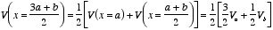
This property immediately suggests a powerful analytical method to
determine the solution of Laplace's equation. If the boundary values of
V are
and
then property 1 can be used to determine the value of the potential at
(a + b)/2:
Next we can determine the value of the potential at x = (3 a
+ b)/4 and at x = (a + 3 b)/4 :
This process can be repeated and V can be calculated in this manner
at any point between x = a and x = b (but not in the
region x > b and x < a).
Property
2:
The solution of Laplace's equation can not have local maxima or
minima. Extreme values must occur at the end points (the boundaries). This is
a direct consequence of property 1.
Property 2 has an important consequence:
a charged particle can not be held in stable equilibrium by electrostatic forces
alone (Earnshaw's Theorem). A particle is in a stable equilibrium
if it is located at a position where the potential has a minimum value. A small
displacement away from the equilibrium position will increase the electrostatic
potential of the particle, and a restoring force will try to move the particle
back to its equilibrium position. However, since there can be no local maxima
or minima in the electrostatic potential, the particle can not be held in stable
equilibrium by just electrostatic forces.
3.1.2. Laplace's Equation in Two Dimensions
In two dimensions the electrostatic potential depends on two variables
x and y. Laplace's equation now becomes
This equation does not have a simple analytical solution as the
one-dimensional Laplace equation does. However, the properties of solutions of
the one-dimensional Laplace equation are also valid for solutions of the
two-dimensional Laplace equation:
Property 1:
The value of
V at a point (x, y) is equal to the average value of
V around this point
where the path integral is along a circle of arbitrary radius, centered at
(x, y) and with radius R.
Property
2:
V has no local maxima or minima; all extremes occur at the
boundaries.
3.1.3. Laplace's Equation in Three Dimensions
In three dimensions the electrostatic potential depends on three variables
x, y, and z. Laplace's equation now becomes
This equation does not have a simple analytical solution as the
one-dimensional Laplace equation does. However, the properties of solutions of
the one-dimensional Laplace equation are also valid for solutions of the
three-dimensional Laplace equation:
Property 1:
The value of
V at a point (x, y, z) is equal to the average value
of V around this point
where the surface integral is across the surface of a sphere of arbitrary
radius, centered at (x,y,z) and with radius
R.
 Figure
3.1. Proof of property 1.
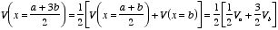
Figure
3.1. Proof of property 1. To proof this property of V consider the electrostatic potential
generated by a point charge q located on the z axis, a distance
r away from the center of a sphere of radius R (see Figure 3.1).
The potential at P, generated by charge q, is equal to
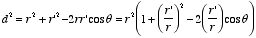
where d is the distance between P and q. Using the
cosine rule we can express d in terms of r, R and
θ
The potential at P due to charge q is therefore equal
to
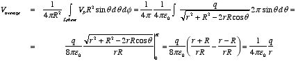
The average potential on the surface of the sphere can be obtained by
integrating

across the surface of the sphere. The average potential is equal to
which is equal to the potential due to q at the center of the
sphere. Applying the principle of superposition it is easy to show that the
average potential generated by a collection of point charges is equal to the net
potential they produce at the center of the sphere.
Property
2:
The electrostatic potential V has no local maxima or minima;
all extremes occur at the boundaries.
Example: Problem
3.3
Find the general solution to Laplace's equation in spherical
coordinates, for the case where V depends only on r. Then do the
same for cylindrical coordinates.
Laplace's equation in spherical
coordinates is given by
If V is only a function of r then
and
Therefore, Laplace's equation can be rewritten as
The solution V of this second-order differential equation must
satisfy the following first-order differential equation:
This differential equation can be rewritten as
The general solution of this first-order differential equation is
where b is a constant. If V = 0 at infinity then b
must be equal to zero, and consequently
Laplace's equation in cylindrical coordinates is
If V is only a function of r then
and
Therefore, Laplace's equation can be rewritten as
The solution V of this second-order differential equation must
satisfy the following first-order differential equation:
This differential equation can be rewritten as
The general solution of this first-order differential equation is
where b is a constant. The constants a and b are
determined by the boundary conditions.
3.1.4. Uniqueness Theorems
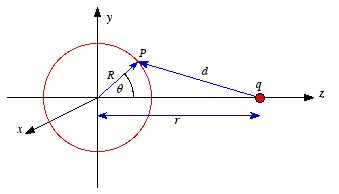
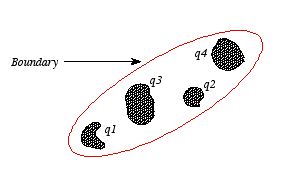
Consider a volume (see Figure 3.2) within which the charge density is
equal to zero. Suppose that the value of the electrostatic potential is
specified at every point on the surface of this volume. The first uniqueness
theorem states that in this case the solution of Laplace's equation is
uniquely defined.
 Figure
3.2. First Uniqueness Theorem
Figure
3.2. First Uniqueness Theorem To proof the first uniqueness theorem we will consider what happens when
there are two solutions V1 and V2 of
Laplace's equation in the volume shown in Figure 3.2. Since
V1 and V2 are solutions of Laplace's
equation we know that
and
Since both V1 and V2 are solutions,
they must have the same value on the boundary. Thus V1 =
V2 on the boundary of the volume. Now consider a third
function V3, which is the difference between
V1 and V2
The function V3 is also a solution of Laplace's equation.
This can be demonstrated easily:
The value of the function V3 is equal to zero on the
boundary of the volume since V1 = V2 there.
However, property 2 of any solution of Laplace's equation states that it can
have no local maxima or minima and that the extreme values of the solution must
occur at the boundaries. Since V3 is a solution of Laplace's
equation and its value is zero everywhere on the boundary of the volume, the
maximum and minimum value of V3 must be equal to zero.
Therefore, V3 must be equal to zero everywhere. This
immediately implies that

everywhere. This proves that there can be no two different functions
V1 and V2 that are solutions of Laplace's
equation and satisfy the same boundary conditions. Therefore, the solution of
Laplace's equation is uniquely determined if its value is a specified function
on all boundaries of the region. This also indicates that it does not matter
how you come by your solution: if (a) it is a solution of Laplace's equation,
and (b) it has the correct value on the boundaries, then it is the right and
only solution.
 Figure
3.3. System with conductors.
Figure
3.3. System with conductors. The first uniqueness theorem can only be applied in those regions that are
free of charge and surrounded by a boundary with a known potential (not
necessarily constant). In the laboratory the boundaries are usually conductors
connected to batteries to keep them at a fixed potential. In many other
electrostatic problems we do not know the potential at the boundaries of the
system. Instead we might know the total charge on the various conductors that
make up the system (note: knowing the total charge on a conductor does not imply
a knowledge of the charge distribution
ρ since it is influenced by
the presence of the other conductors). In addition to the conductors that make
up the system, there might be a charge distribution
ρ filling the
regions between the conductors (see Figure 3.3). For this type of system the
first uniqueness theorem does not apply. The
second uniqueness theorem
states that the electric field is uniquely determined if the total charge on
each conductor is given and the charge distribution in the regions between the
conductors is known.
The proof of the second uniqueness theorem is similar
to the proof of the first uniqueness theorem. Suppose that there are two fields

and

that are solutions of Poisson's equation in the region between the conductors.
Thus

and
where
ρ is the charge density at the point where the electric
field is evaluated. The surface integrals of
and
,
evaluated using a surface that is just outside one of the conductors with charge
Qi, are equal to

.
Thus
The difference between
and
,

,
satisfies the following equations:
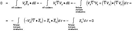
Consider the surface integral of

,
integrated over all surfaces (the surface of all conductors and the outer
surface). Since the potential on the surface of any conductor is constant, the
electrostatic potential associated with
and
must also be constant on the surface of each conductor. Therefore,

will also be constant on the surface of each conductor. The surface integral of

over the surface of conductor
i can be written as
Since the surface integral of
over the surface of conductor
i is equal to zero, the surface integral of
over all conductor surfaces will also be equal to zero. The surface integral of
over the outer surface will also be equal to zero since

on this surface. Thus
The surface integral of
can be rewritten using Green's identity as
where the volume integration is over all space between the conductors and
the outer surface. Since

is always positive, the volume integral of
can only be equal to zero if

everywhere. This implies immediately that

everywhere, and proves the second uniqueness theorem.
3.2. Method of Images
Consider a point charge q held as a distance d above an
infinite grounded conducting plane (see Figure 3.4). The electrostatic
potential of this system must satisfy the following two boundary
conditions:
A direct calculation of the electrostatic potential can not be carried out
since the charge distribution on the grounded conductor is unknown.
Note: the charge distribution on the surface of a grounded
conductor does not need to be zero.
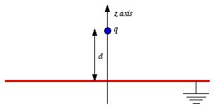 Figure
3.4. Method of images.
Figure
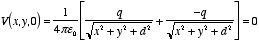
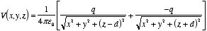
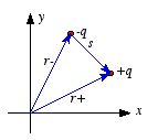
3.4. Method of images. Consider a second system, consisting of two point charges with charges
+q and -q, located at z = d and z =
-d, respectively (see Figure 3.5). The electrostatic potential generated
by these two charges can be calculated directly at any point in space. At a
point P = (x, y, 0) on the xy plane the
electrostatic potential is equal to
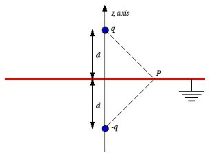 Figure
3.5. Charge and image charge.
Figure
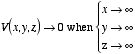
3.5. Charge and image charge.The potential of this system at infinity will approach zero since the
potential generated by each charge will decrease as 1/r with increasing
distance r. Therefore, the electrostatic potential generated by the two
charges shown in Figure 3.5 satisfies the same boundary conditions as the system
shown in Figure 3.4. Since the charge distribution in the region z >
0 (bounded by the xy plane boundary and the boundary at infinity) for the
two systems is identical, the corollary of the first uniqueness theorem states
that the electrostatic potential in this region is uniquely defined. Therefore,
if we find any function that satisfies the boundary conditions and Poisson's
equation, it will be the right answer. Consider a point (x, y,
z) with z > 0. The electrostatic potential at this point can
be calculated easily for the charge distribution shown in Figure 3.5. It is
equal to
Since this solution satisfies the boundary conditions, it must be the
correct solution in the region
z > 0 for the system shown in
Figure 3.4. This technique of using image charges to obtain the electrostatic
potential in some region of space is called the
method of images.
The
electrostatic potential can be used to calculate the charge distribution on the
grounded conductor. Since the electric field inside the conductor is equal to
zero, the boundary condition for

(see Chapter 2) shows that the electric field right outside the conductor is
equal to
where
σ is the surface charge density and

is the unit vector normal to the surface of the conductor. Expressing the
electric field in terms of the electrostatic potential
V we can rewrite
this equation as
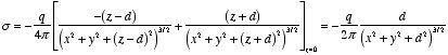
Substituting the solution for V in this equation we find
Only in the last step of this calculation have we substituted z = 0.
The induced charge distribution is negative and the charge density is greatest
at (x = 0, y = 0, z = 0). The total charge on the
conductor can be calculated by surface integrating of σ:
where

.
Substituting the expression for
σ in the integral we
obtain
As a result of the induced surface charge on the conductor, the point
charge q will be attracted towards the conductor. Since the
electrostatic potential generated by the charge image-charge system is the same
as the charge-conductor system in the region where z > 0, the
associated electric field (and consequently the force on point charge q)
will also be the same. The force exerted on point charge q can be
obtained immediately by calculating the force exerted on the point charge by the
image charge. This force is equal to

There is however one important difference between the image-charge system
and the real system. This difference is the total electrostatic energy of the
system. The electric field in the image-charge system is present everywhere,
and the magnitude of the electric field at (
x,
y,
z) will
be the same as the magnitude of the electric field at (
x,
y,
-
z). On the other hand, in the real system the electric field will only
be non zero in the region with
z > 0. Since the electrostatic energy
of a system is proportional to the volume integral of

the electrostatic energy of the real system will be 1/2 of the electrostatic
energy of the image-charge system (only 1/2 of the total volume has a non-zero
electric field in the real system). The electrostatic energy of the
image-charge system is equal to
The electrostatic energy of the real system is therefore equal to
The electrostatic energy of the real system can also be obtained by
calculating the work required to be done to assemble the system. In order to
move the charge q to its final position we will have to exert a force
opposite to the force exerted on it by the grounded conductor. The work done to
move the charge from infinity along the z axis to z = d is
equal to
which is identical to the result obtained using the electrostatic potential
energy of the image-charge system.
Example: Example 3.2 + Problem
3.7
A point charge q is situated a distance s from the
center of a grounded conducting sphere of radius R (see Figure
3.6).
a) Find the potential everywhere.
b) Find the induced surface charge
on the sphere, as function of q. Integrate this to get the total induced
charge.
c) Calculate the electrostatic energy of this
configuration.
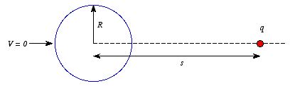 Figure
3.6. Example 3.2 + Problem 3.7.
Figure
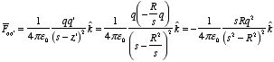
3.6. Example 3.2 + Problem 3.7.a) Consider a system consisting of two charges q and q',
located on the z axis at z = s and z = z',
respectively. If the potential produced by this system is identical everywhere
to the potential produced by the system shown in Figure 3.6 then the position of
point charge q' must be chosen such that the potential on the surface of
a sphere of radius R, centered at the origin, is equal to zero (in this
case the boundary conditions for the potential generated by both systems are
identical).
We will start with determining the correct position of point
charge q'. The electrostatic potential at P (see Figure 3.7) is
equal to
This equation can be rewritten as

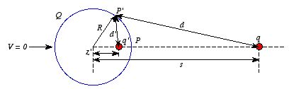 Figure
3.7. Image-charge system.
Figure
3.7. Image-charge system.The electrostatic potential at Q is equal to
This equation can be rewritten as
Combining the two expression for q' we obtain
or
This equation can be rewritten as
The position of the image charge is equal to
The value of the image charge is equal to
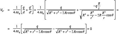
Now consider an arbitrary point P' on the circle. The distance
between P' and charge q is d and the distance between
P' and charge q' is equal to d'. Using the cosine rule
(see Figure 3.7) we can express d and d' in terms of R,
s, and θ:
The electrostatic potential at P' is equal to
Thus we conclude that the configuration of charge and image charge produces
an electrostatic potential that is zero at any point on a sphere with radius
R and centered at the origin. Therefore, this charge configuration
produces an electrostatic potential that satisfies exactly the same boundary
conditions as the potential produced by the charge-sphere system. In the region
outside the sphere, the electrostatic potential is therefore equal to the
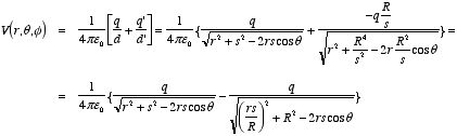
electrostatic potential produced by the charge and image charge. Consider an
arbitrary point

.
The distance between this point and charge
q is
d and the distance
between this point and charge
q' is equal to
d'. These distances
can be expressed in terms of
r,
s, and
θ using the
cosine rule:
The electrostatic potential at
will therefore be equal to
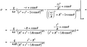
b) The surface charge density
σ on the sphere can be obtained
from the boundary conditions of
where we have used the fact that the electric field inside the sphere is
zero. This equation can be rewritten as
Substituting the general expression for V into this equation we
obtain
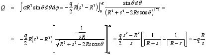
The total charge on the sphere can be obtained by integrating σ
over the surface of the sphere. The result is
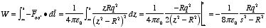
c) To obtain the electrostatic energy of the system we can determine the
work it takes to assemble the system by calculating the path integral of the
force that we need to exert in charge q in order to move it from infinity
to its final position (z = s). Charge q will feel an
attractive force exerted by the induced charge on the sphere. The strength of
this force is equal to the force on charge q exerted by the image charge
q'. This force is equal to
The force that we must exert on
q to move it from infinity to its
current position is opposite to

.
The total work required to move the charge is therefore equal to
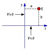
Example: Problem 3.10
Two semi-infinite grounded
conducting planes meet at right angles. In the region between them, there is a
point charge q, situated as shown in Figure 3.8. Set up the image
configuration, and calculate the potential in this region. What charges do you
need, and where should they be located? What is the force on q? How
much work did it take to bring q in from infinity?
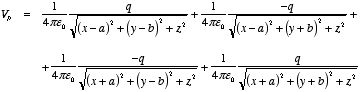
Consider the
system of four charges shown in Figure 3.9. The electrostatic potential
generated by this charge distribution is zero at every point on the yz
plane and at every point on the xz plane. Therefore, the electrostatic
potential generated by this image charge distribution satisfies the same
boundary conditions as the electrostatic potential of the original system. The
potential generated by the image charge distribution in the region where
x > 0 and y > 0 will be identical to the potential of the
original system. The potential at a point P = (x, y,
z) is equal to
 Figure
3.8. Problem
3.10.
Figure
3.8. Problem
3.10.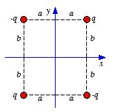 Figure
3.9. Image charges for problem 3.10.
Figure
3.9. Image charges for problem 3.10.The force exerted on q can be obtained by calculating the force
exerted on q by the image charges. The total force is equal to the
vector sum of the forces exerted by each of the three image charges. The force
exerted by the image charge located at (-a, b, 0) is directed
along the negative x axis and is equal to
The force exerted by the image charge located at (a, -b, 0)
is directed along the negative y axis and is equal to
The force exerted by the image charge located at (-a, -b, 0)
is directed along the vector connecting (-a, -b, 0) and (a,
b, 0) and is equal to
The total force on charge
q is the vector sum of

,

and

:
The electrostatic potential energy of the system can, in principle, be
obtained by calculating the path integral of

between infinity and (
a,
b, 0). However, this is not trivial
since the force
is a rather complex function of
a and
b. An easier technique is
to calculate the electrostatic potential energy of the system with charge and
image charges. The potential energy of this system is equal to
However, in the real system the electric field is only non-zero in the
region where x > 0 and y > 0. Therefore, the total
electrostatic potential energy of the real system is only 1/4 of the total
electrostatic potential energy of the image charge system. Thus
3.3. Separation of Variables
3.3.1. Separation of variables: Cartesian coordinates
A powerful technique very frequently used to solve partial differential
equations is
separation of variables. In this section we will
demonstrate the power of this technique by discussing several
examples.
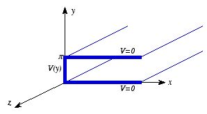
Example: Example 3.3 (Griffiths) Two infinite,
grounded, metal plates lie parallel to the
xz plane, one at
y = 0,
the other at
y =
π (see Figure 3.10). The left end, at
x = 0, is closed off with an infinite strip insulated from the two plates
and maintained at a specified potential

.
Find the potential inside this "slot".
 Figure
3.10. Example 3.3 (Griffiths).
Figure
3.10. Example 3.3 (Griffiths). The electrostatic potential in the slot must satisfy the three-dimensional
Laplace equation. However, since V does not have a z dependence,
the three-dimensional Laplace equation reduces to the two-dimensional Laplace
equation:
The boundary conditions for the solution of Laplace's equation
are:
1. V(x, y = 0) = 0 (grounded bottom
plate).
2. V(x, y = π) = 0 (grounded top
plate).
3. V(x = 0, y) =
V0(y) (plate at x = 0).
4. V
→ 0 when x → ∞.
These four boundary conditions
specify the value of the potential on all boundaries surrounding
the slot and are therefore sufficient to uniquely determine the solution of
Laplace's equation inside the slot. Therefore, if we find one solution of
Laplace's equation satisfying these boundary conditions than it must be the
correct one. Consider solutions of the following form:
If this is a solution of the two-dimensional Laplace equation than we must
require that
This equation can be rewritten as
The first term of the left-hand side of this equation depends only on
x while the second term depends only on y. Therefore, if this
equation must hold for all x and y in the slot we must require
that
and
The differential equation for X can be rewritten as
If C1 is a negative number than this equation can be
rewritten as
where k2 = -C1 . The most general
solution of this equation is
However, this function is an oscillatory function and does not satisfy
boundary condition # 4, which requires that V approaches zero when
x approaches infinity. We therefore conclude that C1
can not be a negative number. If C1 is a positive
number then the differential equation for X can be written as
The most general solution of this equation is
This solution will approach zero when x approaches infinity if
A = 0. Thus
The solution for Y can be obtained by solving the following
differential equation:
The most general solution of this equation is
Therefore, the general solution for the electrostatic potential
V(x,y) is equal to
where we have absorbed the constant B into the constants C
and D. The constants C and D must be chosen such that the
remaining three boundary conditions (1, 2, and 3) are satisfied. The first
boundary condition requires that V(x, y = 0) = 0:
which requires that C = 0. The second boundary condition requires
that V(x, y = π) = 0:
which requires that

.
This condition limits the possible values of
k to positive
integers:
Note: negative values of k are not allowed since exp(-kx)
approaches zero at infinity only if k > 0. To satisfy boundary
condition # 3 we must require that
This last expression suggests that the only time at which we can find a
solution of Laplace's equation that satisfies all four boundary conditions has
the form

is when

happens to have the form

.
However, since
k can take on an infinite number of values, there will be
an infinite number of solutions of Laplace's equation satisfying boundary
conditions # 1, # 2 and # 4. The most general form of the solution of Laplace's
equation will be a linear superposition of all possible solutions.
Thus
Boundary condition # 3 can now be written as
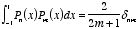
Multiplying both sides by sin(ny) and integrating each side between
y = 0 and y = π we obtain
The integral on the left-hand side of this equation is equal to zero for
all values of k except k = n. Thus
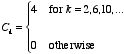
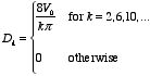
The coefficients Dk can thus be calculated
easily:
The coefficients
Dk are called the
Fourier
coefficients of
.
The solution of Laplace's equation in the slot is therefore equal to
where
Now consider the special case in which
.
In this case the coefficients
Dk are equal to
The solution of Laplace's equation is thus equal to
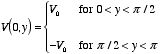
Example: Problem 3.12 Find the potential in the infinite
slot of Example 3.3 (Griffiths) if the boundary at
x = 0 consists to two
metal stripes: one, from
y = 0 to
y = π/2, is held at
constant potential

,
and the other, from
y = π/2 to
y = π is at potential

.
The
boundary condition at
x = 0 is
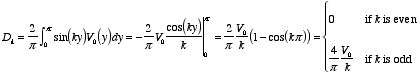
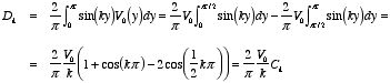
The Fourier coefficients of the function
are equal to
The values for the first four C coefficients are
It is easy to see that Ck + 4 =
Ck and therefore we conclude that
The Fourier coefficients Ck are thus equal to
The electrostatic potential is thus equal to
Example: Problem 3.13 For the infinite slot (Example 3.3
Griffiths) determine the charge density

on the strip at
x=0, assuming it is a conductor at constant potential

.
The
electrostatic potential in the slot is equal to
The charge density at the plate at x = 0 can be obtained using the
boundary condition for the electric field at a boundary:
where

is directed along the positive
x axis. Since

this boundary condition can be rewritten as
Differentiating V(x,y) with respect to x we
obtain
At the x = 0 boundary we obtain
The charge density σ on the x = 0 strip is therefore
equal to
Example: Double infinite slots
The slot of example 3.3 in
Griffiths and its mirror image at negative x are separated by an
insulating strip at x = 0. If the charge density σ(y)
on the dividing strip is given, determine the potential in the slot.
The
boundary condition at x = 0 requires that
where

is directed along the positive
x axis. Here we have used the symmetry of
the configuration which requires that the electric field in the region
x
< 0 is the mirror image of the field in the region
x > 0. Since
this boundary condition can be rewritten as
We will first determine the potential in the x > 0 region.
Following the same procedure as in Example 3 we obtain for the electrostatic
potential
where the constants Dk must be chosen such that the
boundary condition at x = 0 is satisfied. This requires that
Thus
The constants
Dk can be determined by multiplying both
sides of this equation with

and integrating both sides with respect to
y between
y = 0 and
y = π. The result is
The constants Ck are thus equal to
The electrostatic potential is thus equal to
3.3.2. Separation of variables: spherical coordinates
Consider a spherical symmetric system. If we want to solve Laplace's
equation it is natural to use spherical coordinates. Assuming that the system
has azimuthal symmetry
(

)
Laplace's equation reads
Multiplying both sides by r2 we obtain
Consider the possibility that the general solution of this equation is the
product of a function

,
which depends only on the distance
r, and a function

,
which depends only on the angle
θ:
Substituting this "solution" into Laplace's equation we obtain
Dividing each term of this equation by

we obtain
The first term in this expression depends only on the distance r
while the second term depends only on the angle θ. This equation
can only be true for all r and θ if
and
Consider a solution for R of the following form:
where A and k are arbitrary constants. Substituting this
expression in the differential equation for R(r) we
obtain
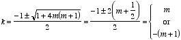
Therefore, the constant k must satisfy the following
relation:
This equation gives us the following expression for k
The general solution for
is thus given by
where A and B are arbitrary constants.
The angle
dependent part of the solution of Laplace's equation must satisfy the following
equation
The solutions of this equation are known as the
Legendre polynomial

.
The Legendre polynomials have the following properties:
1. if
m
is even:

2.
if
m is odd:

3.

for all
m 4.
or
Combining
the solutions for
and
we obtain the most general solution of Laplace's equation in a spherical
symmetric system with azimuthal symmetry:
Example: Problem 3.18
The potential at the surface of a
sphere is given by
where
k is some constant. Find the potential inside and outside the
sphere, as well as the surface charge density

on the sphere. (Assume that there is no charge inside or outside of the
sphere.)
The most general solution of Laplace's equation in spherical
coordinates is
First consider the region inside the sphere (
r <
R). In
this region

since otherwise

would blow up at
r = 0. Thus
The potential at r = R is therefore equal to
Using trigonometric relations we can rewrite

as
Substituting this expression in the equation for

we obtain
This equation immediately shows that

unless

.
If
then
The electrostatic potential inside the sphere is therefore equal
to
Now consider the region outsider the sphere (
r >
R). In
this region

since otherwise
would blow up at infinity. The solution of Laplace's equation in this region is
therefore equal to
The potential at r = R is therefore equal to
The equation immediately shows that

except when
.
If
then
The electrostatic potential outside the sphere is thus equal to
The charge density on the sphere can be obtained using the boundary
conditions for the electric field at a boundary:
Since
this boundary condition can be rewritten as
The first term on the left-hand side of this equation can be calculated
using the electrostatic potential just obtained:
In the same manner we obtain
Therefore,
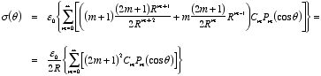
The charge density on the sphere is thus equal to
Example: Problem 3.19 Suppose the potential

at the surface of a sphere is specified, and there is no charge inside or
outside the sphere. Show that the charge density on the sphere is given
by
where
Most of the solution of this problem is very similar to the solution
of Problem 3.18. First consider the electrostatic potential inside the sphere.
The electrostatic potential in this region is given by
and the boundary condition is
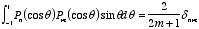
The coefficients

can be determined by multiplying both sides of this equation by

and integrating with respect to
θ between
θ = 0 and
θ = π:
Thus
In the region outside the sphere the electrostatic potential is given
by
and the boundary condition is
The coefficients

are given by
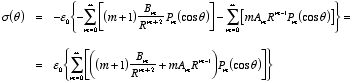
The charge density
on the surface of the sphere is equal to
Differentiating
with respect to
r in the region
r >
R we
obtain
Differentiating
with respect to
r in the region
r <
R we
obtain
The charge density is therefore equal to
Substituting the expressions for
and
into this equation we obtain
where
Example: Problem 3.23 Solve Laplace's equation by
separation of variables in
cylindrical coordinates, assuming there is no
dependence on
z (cylindrical symmetry). Make sure that you find
all solutions to the radial equation. Does your result accommodate the
case of an infinite line charge?
For a system with cylindrical symmetry
the electrostatic potential does not depend on
z. This immediately
implies that

.
Under this assumption Laplace's equation reads
Consider as a possible solution of V:
Substituting this solution into Laplace's equation we obtain
Multiplying each term in this equation by
r2 and dividing
by

we obtain
The first term in this equation depends only on r while the second
term in this equation depends only on φ. This equation can
therefore be only valid for every r and every φ if each term
is equal to a constant. Thus we require that
and
First consider the case in which

.
The differential equation for

can be rewritten as
The most general solution of this differential solution is
However, in cylindrical coordinates we require that any solution for a
given
φ is equal to the solution for
φ + 2
π.
Obviously this condition is not satisfied for this solution, and we conclude
that

.
The differential equation for
can be rewritten as
The most general solution of this differential solution is
The condition that

requires that
m is an integer. Now consider the radial function
.
We will first consider the case in which

.
Consider the following solution for
:
Substituting this solution into the previous differential equation we
obtain
Therefore, the constant k can take on the following two
values:
The most general solution for
under the assumption that

is therefore
Now consider the solutions for
when

.
In this case we require that
or
This equation can be rewritten as
If

then the solution of this differential equation is
If

then the solution of this differential equation is
Combining the solutions obtained for

with the solutions obtained for

we conclude that the most general solution for
is given by
Therefore, the most general solution of Laplace's equation for a system
with cylindrical symmetry is
Example: Problem 3.25
A charge density
is glued over the surface of an infinite cylinder of radius
R. Find
the potential inside and outside the cylinder.
The electrostatic
potential can be obtained using the general solution of Laplace's equation for a
system with cylindrical symmetry obtained in Problem 3.24. In the region inside
the cylinder the coefficient

must be equal to zero since otherwise

would blow up at

.
For the same reason

.
Thus
In the region outside the cylinder the coefficients

must be equal to zero since otherwise
would blow up at infinity. For the same reason
.
Thus
Since
must approach 0 when
r approaches infinity, we must also require that

is equal to 0. The charge density on the surface of the cylinder is equal
to
Differentiating
in the region
r >
R and setting
r =
R we
obtain
Differentiating
in the region
r <
R and setting
r =
R we
obtain
The charge density on the surface of the cylinder is therefore equal
to
Since the charge density is proportional to

we can conclude immediately that

for all

and that

for all
except

.
Therefore
This requires that
A second relation between

and

can be obtained using the condition that the electrostatic potential is
continuous at any boundary. This requires that
Thus
and
We now have two equations with two unknown,
and
,
which can be solved with the following result:
and
The electrostatic potential inside the cylinder is thus equal to
The electrostatic potential outside the cylinder is thus equal to
Example: Problem 3.37 A conducting sphere of radius
a, at potential

,
is surrounded by a thin concentric spherical shell of radius
b, over
which someone has glued a surface charge
where

is a constant.
a) Find the electrostatic potential in each
region:
i)
r >
b ii)
a <
r <
bb) Find the induced surface charge
on the conductor.
c) What is the total charge of the system? Check that your
answer is consistent with the behavior of
V at large
r.
a) The system has spherical symmetry and we can therefore use
the most general solution of Laplace's equation in spherical
coordinates:
In the region inside the sphere

since otherwise

would blow up at
r = 0. Therefore
The boundary condition for
is that it is equal to
at
r =
a:
This immediately shows that

for all
except

:
The electrostatic potential inside the sphere is thus given by
which should not come as a surprise.
In the region outside the shell

since otherwise
would blow up at infinity. Thus
In the region between the sphere and the shell the most general solution
for

is given by
The boundary condition for

at
r =
a is
This equation can only be satisfied if
The requirement that the electrostatic potential is continuous at r
= b requires that
or
This condition can be rewritten as
The other boundary condition for the electrostatic potential at r =
b is that it must produce the charge distribution given in the problem.
This requires that
This condition is satisfied if
Substituting the relation between the various coefficients obtained by
applying the continuity condition we obtain
These equations show that
Using these values for

we can show that
The boundary condition for V at r = a shows
that
These values for

immediately fix the values for

:
The potential in the region outside the shell is therefore equal
to
The potential in the region between the sphere and the shell is equal
to
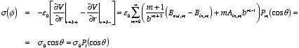
b) The charge density on the surface of the sphere can be found by
calculating the slope of the electrostatic potential at this surface:
c) The total charge on the sphere is equal to
The total charge on the shell is equal to zero. Therefore the total charge
of the system is equal to
The electrostatic potential at large distances will therefore be
approximately equal to
This is equal to limit of the exact electrostatic potential when

.
3.4. Multipole Expansions
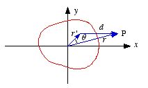
Consider a given charge distribution ρ. The potential at a
point P (see Figure 3.11) is equal to
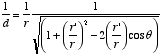
where d is the distance between P and a infinitesimal segment
of the charge distribution. Figure 3.11 shows that d can be written as a
function of r, r' and θ:
 Figure
3.11. Charge distribution ρ.
Figure
3.11. Charge distribution ρ.This equation can be rewritten as
At large distances from the charge distribution

and consequently

.
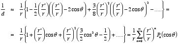
Using the following expansion for

:
we can rewrite 1/d as
Using this expansion of 1/d we can rewrite the electrostatic
potential at P as
This expression is valid for all
r (not only

).
However, if
then the potential at
P will be dominated by the first non-zero term in
this expansion. This expansion is known as the
multipole expansion. In
the limit of
only the first terms in the expansion need to be considered:
The first term in this expression, proportional to 1/r, is called
the monopole term. The second term in this expression, proportional to
1/r2, is called the dipole term. The third term in
this expression, proportional to 1/r3, is called the
quadrupole term.
3.4.1. The monopole term.
If the total charge of the system is non zero then the electrostatic
potential at large distances is dominated by the monopole term:
where
Q is the total charge of the charge distribution.
The
electric field associated with the monopole term can be obtained by calculating
the gradient of

:
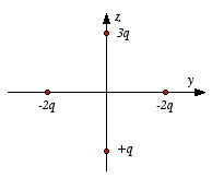
3.4.2. The dipole term.
If the total charge of the charge distribution is equal to zero (Q
= 0) then the monopole term in the multipole expansion will be equal to zero.
In this case the dipole term will dominate the electrostatic potential at large
distances
Since
θ is the angle between

and

we can rewrite

as
The electrostatic potential at P can therefore be rewritten
as
In this expression

is the
dipole moment of the charge distribution which is defined
as
The electric field associated with the dipole term can be obtained by
calculating the gradient of

:
Example
Consider a system of two point charges shown in
Figure 3.12. The total charge of this system is zero, and therefore the
monopole term is equal to zero. The dipole moment of this system is equal
to
where

is the vector pointing from -
q to +
q.
The dipole moment of
a charge distribution depends on the origin of the coordinate system chosen.
Consider a coordinate system
S and a charge distribution
ρ.
The dipole moment of this charge distribution is equal to
A second coordinate system
S' is displaced by

with respect to
S:
The dipole moment of the charge distribution in S' is equal
to
This equation shows that if the total charge of the system is zero
(Q = 0) then the dipole moment of the charge distribution is independent
of the choice of the origin of the coordinate system.
 Figure
3.12. Electric dipole moment.
Figure
3.12. Electric dipole moment. Example: Problem 3.40 A thin insulating rod, running from
z = -
a to
z = +
a, carries the following line
charges:
a)

b)

c)

In
each case, find the leading term in the multipole expansion of the
potential.
a) The total charge on the rod is equal to
Since

,
the monopole term will dominate the electrostatic potential at large distances.
Thus
b) The total charge on the rod is equal to zero. Therefore, the
electrostatic potential at large distances will be dominated by the dipole term
(if non-zero). The dipole moment of the rod is equal to
Since the dipole moment of the rod is not equal to zero, the dipole term
will dominate the electrostatic potential at large distances.
Therefore
c) For this charge distribution the total charge is equal to zero and the
dipole moment is equal to zero. The electrostatic potential of this charge
distribution is dominated by the quadrupole term.
The electrostatic potential at large distance from the rod will be equal
to
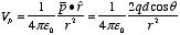
Example: Problem 3.27
Four particles (one of charge
q, one of charge 3q, and two of charge -2q) are placed as
shown in Figure 3.12, each a distance d from the origin. Find a simple
approximate formula for the electrostatic potential, valid at a point P
far from the origin.
The total charge of the system is equal to zero and
therefore the monopole term in the multipole expansion is equal to zero. The
dipole moment of this charge distribution is equal to
The Cartesian coordinates of P are
The scalar product between

and

is therefore
The electrostatic potential at P is therefore equal to
 Figure
3.13. Problem 3.27.
Figure
3.13. Problem 3.27. Example: Problem 3.38 A charge
Q is distributed
uniformly along the
z axis from
z = -
a to
z
=
a. Show that the electric potential at a point

is given by
for r > a.
The charge density along this segment
of the z axis is equal to
Therefore, the nth moment of the charge distribution is equal
to
This equation immediately shows that
The electrostatic potential at P is therefore equal to