Chapter 2. Electrostatics
2.1. The Electrostatic Field
To calculate the force exerted by some electric charges,
q1,
q2,
q3, ... (
the
source charges) on another charge
Q (
the test charge) we can
use the
principle of superposition. This principle states that the
interaction between any two charges is completely unaffected by the presence of
other charges. The force exerted on
Q by
q1,
q2, and
q3 (see Figure 2.1) is therefore
equal to the vector sum of the force

exerted by
q1 on
Q, the force

exerted by
q2 on
Q, and the force

exerted by
q3 on
Q.
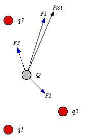 Figure
2.1. Superposition of forces.
Figure
2.1. Superposition of forces. The force exerted by a charged particle on another charged particle depends
on their separation distance, on their velocities and on their accelerations.
In this Chapter we will consider the special case in which the source charges
are stationary.
The
electric field produced by stationary source
charges is called and
electrostatic field. The electric field at a
particular point is a vector whose magnitude is proportional to the total force
acting on a test charge located at that point, and whose direction is equal to
the direction of the force acting on a positive test charge. The electric field

,
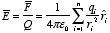
generated by a collection of source charges, is defined as
where

is the total electric force exerted by the source charges on the test charge
Q. It is assumed that the test charge
Q is small and therefore
does not change the distribution of the source charges. The total force exerted
by the source charges on the test charge is equal to
The electric field generated by the source charges is thus equal
to
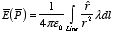
In most applications the source charges are not discrete, but are
distributed continuously over some region. The following three different
distributions will be used in this course:
1.
line charge λ:
the charge per unit length.
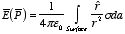
2.
surface charge σ: the charge
per unit area.
3.
volume charge ρ: the charge per unit
volume.
To calculate the electric field at a point

generated by these charge distributions we have to replace the summation over
the discrete charges with an integration over the continuous charge
distribution:
1. for a line charge:
2.
for a surface charge:
3.
for a volume charge:
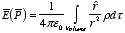
Here

is the unit vector from a segment of the charge distribution to the point
at which we are evaluating the electric field, and
r is the distance
between this segment and point
.
Example:
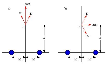
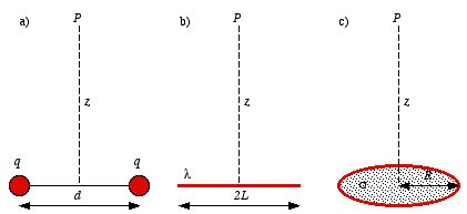
Problem 2.2a) Find the electric field (magnitude and direction) a
distance
z above the midpoint between two equal charges
q a
distance
d apart. Check that your result is consistent with what you
would expect when
z »
d.
b) Repeat part a), only this time
make he right-hand charge
-q instead of +
q.
 Figure
2.2. Problem 2.2
Figure
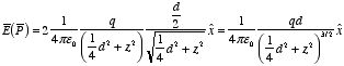
2.2. Problem 2.2a) Figure 2.2a shows that the x components of the electric fields
generated by the two point charges cancel. The total electric field at P
is equal to the sum of the z components of the electric fields
generated by the two point charges:
When z » d this equation becomes approximately equal
to
which is the Coulomb field generated by a point charge with charge
2q.
b) For the electric fields generated by the point charges of
the charge distribution shown in Figure 2.2b the z components cancel.
The net electric field is therefore equal to
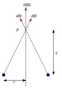
Example: Problem 2.5
Find the electric field a distance
z above the center of a circular loop of radius r which carries a
uniform line charge λ.
 Figure
2.3. Problem 2.5.
Figure
2.3. Problem 2.5. Each segment of the loop is located at the same distance from P (see
Figure 2.3). The magnitude of the electric field at P due to a segment
of the ring of length dl is equal to
When we integrate over the whole ring, the horizontal components of the
electric field cancel. We therefore only need to consider the vertical
component of the electric field generated by each segment:
The total electric field generated by the ring can be obtained by
integrating dEz over the whole ring:
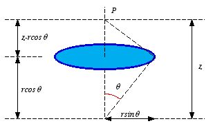
Example: Problem 2.7
Find the electric field a distance
z from the center of a spherical surface of radius R, which
carries a uniform surface charge density σ. Treat the case z
< R (inside) as well as z > R (outside). Express
your answer in terms of the total charge q on the surface.
 Figure
2.4. Problem 2.7.
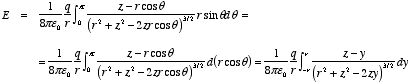
Figure
2.4. Problem 2.7. Consider a slice of the shell centered on the z axis (see Figure
2.4). The polar angle of this slice is θ and its width is
dθ. The area dA of this ring is
The total charge on this ring is equal to
where q is the total charge on the shell. The electric field
produced by this ring at P can be calculated using the solution of
Problem 2.5:
The total field at P can be found by integrating dE with
respect to θ:
This integral can be solved using the following relation:
Substituting this expression into the integral we obtain:
Outside the shell, z > r and consequently the electric
field is equal to
Inside the shell, z < r and consequently the electric
field is equal to
Thus the electric field of a charged shell is zero inside the shell. The
electric field outside the shell is equal to the electric field of a point
charge located at the center of the shell.
2.2. Divergence and Curl of Electrostatic
Fields
The electric field can be graphically represented using field lines. The
direction of the field lines indicates the direction in which a positive test
charge moves when placed in this field. The density of field lines per unit
area is proportional to the strength of the electric field. Field lines
originate on positive charges and terminate on negative charges. Field lines
can never cross since if this would occur, the direction of the electric field
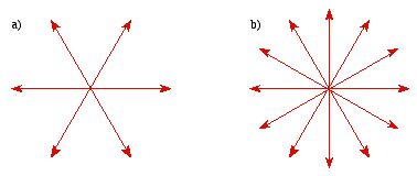
at that particular point would be undefined. Examples of field lines produced
by positive point charges are shown in Figure 2.5.
 Figure
2.5. a) Electric field lines generated by a positive point charge with charge
q. b) Electric field lines generated by a positive point charge with
charge 2q.
Figure
2.5. a) Electric field lines generated by a positive point charge with charge
q. b) Electric field lines generated by a positive point charge with
charge 2q. The flux of electric field lines through any surface is proportional to the
number of field lines passing through that surface. Consider for example a
point charge
q located at the origin. The electric flux

through a sphere of radius
r, centered on the origin, is equal
to
Since the number of field lines generated by the charge
q depends
only on the magnitude of the charge, any arbitrarily shaped surface that
encloses
q will intercept the same number of field lines. Therefore the
electric flux through any surface that encloses the charge
q is equal to

.
Using the principle of superposition we can extend our conclusion easily to
systems containing more than one point charge:
We thus conclude that for an arbitrary surface and arbitrary charge
distribution
where
Qenclosed is the total charge enclosed by the
surface. This is called
Gauss's law. Since this equation involves an
integral it is also called
Gauss's law in integral form.
Using the
divergence theorem the electric flux

can be rewritten as
We can also rewrite the enclosed charge Qencl in terms of
the charge density ρ:
Gauss's law can thus be rewritten as
Since we have not made any assumptions about the integration volume this
equation must hold for any volume. This requires that the integrands are
equal:
This equation is called
Gauss's law in differential
form.
Gauss's law in differential form can also be obtained directly
from Coulomb's law for a charge distribution

:
where

.
The divergence of

is equal to
which is Gauss's law in differential form. Gauss's law in integral form
can be obtained by integrating

over the volume
V:
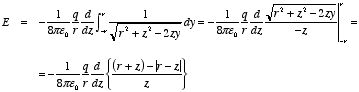
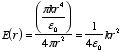
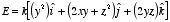
Example: Problem 2.42
If the electric field in some region
is given (in spherical coordinates) by the expression
where A and B are constants, what is the charge density
ρ?
The charge density ρ can be obtained from the
given electric field, using Gauss's law in differential form:
2.2.1. The curl of E
Consider a charge distribution ρ(r). The electric
field at a point P generated by this charge distribution is equal
to
where
.
The curl of

is equal to
However,

for every vector

and we thus conclude that
2.2.2. Applications of Gauss's law
Although Gauss's law is always true it is only a useful tool to calculate
the electric field if the charge distribution is symmetric:
1. If the
charge distribution has spherical symmetry, then Gauss's law can be used
with concentric spheres as Gaussian surfaces.
2. If the charge
distribution has cylindrical symmetry, then Gauss's law can be used with
coaxial cylinders as Gaussian surfaces.
3. If the charge distribution has
plane symmetry, then Gauss's law can be used with pill boxes as Gaussian
surfaces.
Example: Problem 2.12
Use Gauss's law to find the
electric field inside a uniformly charged sphere (charge density ρ)
of radius R.
The charge distribution has spherical symmetry
and consequently the Gaussian surface used to obtain the electric field will be
a concentric sphere of radius r. The electric flux through this surface
is equal to
The charge enclosed by this Gaussian surface is equal to
Applying Gauss's law we obtain for the electric field:
Example: Problem 2.14
Find the electric field inside a
sphere which carries a charge density proportional to the distance from the
origin: ρ = k r, for some constant
k.
The charge distribution has spherical symmetry and we will
therefore use a concentric sphere of radius r as a Gaussian surface.
Since the electric field depends only on the distance r, it is constant
on the Gaussian surface. The electric flux through this surface is therefore
equal to
The charge enclosed by the Gaussian surface can be obtained by integrating
the charge distribution between r' = 0 and r' =
r:
Applying Gauss's law we obtain:
or
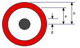
Example: Problem 2.16 A long coaxial cable carries a
uniform (positive) volume charge density
ρ on the inner cylinder
(radius
a), and uniform surface charge density on the outer cylindrical
shell (radius
b). The surface charge is negative and of just the right
magnitude so that the cable as a whole is neutral. Find the electric field in
each of the three regions: (1) inside the inner cylinder (
r <
a), (2) between the cylinders (
a <
r <
b), (3)
outside the cable (
b <
r).
The charge distribution has
cylindrical symmetry and to apply Gauss's law we will use a cylindrical Gaussian
surface. Consider a cylinder of radius
r and length
L. The
electric field generated by the cylindrical charge distribution will be radially
directed. As a consequence, there will be no electric flux going through the
end caps of the cylinder (since here

).
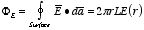
The total electric flux through the cylinder is equal to
The enclosed charge must be calculated separately for each of the three
regions:
1.
r <
a:

2.
a
<
r <
b:

3.
b
<
r:

Applying
Gauss's law we find
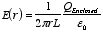
Substituting the calculated
Qencl for the three regions
we obtain
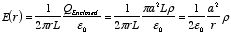
1.
r <
a:
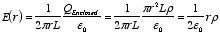
.
2.
a
<
r <
b:
3.
b
<
r  Example:
Problem 2.18
Example:
Problem 2.18 Two spheres, each of radius
R and carrying uniform
charge densities of +
ρ and -
ρ, respectively, are placed
so that they partially overlap (see Figure 2.6). Call the vector from the
negative center to the positive center

.
Show that the field in the region of overlap is constant and find its
value.
To calculate the total field generated by this charge
distribution we use the principle of superposition. The electric field
generated by each sphere can be obtained using Gauss' law (see Problem 2.12).
Consider an arbitrary point in the overlap region of the two spheres (see Figure
2.7). The distance between this point and the center of the negatively charged
sphere is
r-. The distance between this point and the center
of the positively charged sphere is
r+. Figure 2.7 shows that
the vector sum of
and

is equal to

.
Therefore,

The total electric field at this point in the overlap region is the vector
sum of the field due to the positively charged sphere and the field due to the
negatively charged sphere:

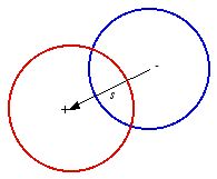 Figure
2.6. Problem
2.18.
Figure
2.6. Problem
2.18.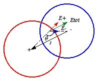 Figure
2.7. Calculation of Etot.
Figure
2.7. Calculation of Etot.The minus sign in front of
shows that the electric field generated by the negatively charged sphere is
directed opposite to
.
Using the relation between
and
obtained from Figure 2.7 we can rewrite

as
which shows that the field in the overlap region is homogeneous and
pointing in a direction opposite to

.
2.3. The Electric Potential
The requirement that the curl of the electric field is equal to zero
limits the number of vector functions that can describe the electric field. In
addition, a theorem discussed in Chapter 1 states that any vector function whose
curl is equal to zero is the gradient of a scalar function. The scalar function
whose gradient is the electric field is called the electric potential
V and it is defined as
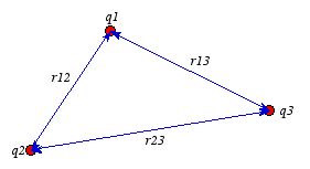
Taking the line integral of

between point
a and point
b we obtain
Taking a to be the reference point and defining the potential to be
zero there, we obtain for V(b)
The choice of the reference point a of the potential is arbitrary.
Changing the reference point of the potential amounts to adding a constant to
the potential:
where K is a constant, independent of b, and equal
to
However, since the gradient of a constant is equal to zero
Thus, the electric field generated by V' is equal to the electric
field generated by V. The physical behavior of a system will depend only
on the difference in electric potential and is therefore independent of the
choice of the reference point. The most common choice of the reference point in
electrostatic problems is infinity and the corresponding value of the potential
is usually taken to be equal to zero:
The unit of the electrical potential is the Volt (V, 1V = 1
Nm/C).
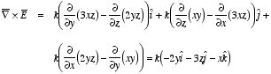
Example: Problem 2.20 One of these is an impossible
electrostatic field. Which
one?
a)
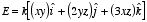
b)
Here,
k is a constant with the appropriate units. For the
possible one,
find the potential, using the origin as your reference point. Check your answer
by computing
.
a) The
curl of this vector function is equal to
Since the curl of this vector function is not equal to zero, this vector
function can not describe an electric field.
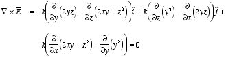
b) The curl of this vector
function is equal to
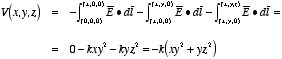
Since the curl of this vector function is equal to zero it can describe an
electric field. To calculate the electric potential
V at an arbitrary
point (
x,
y,
z), using (0, 0, 0) as a reference point, we
have to evaluate the line integral of

between (0, 0, 0) and (
x,
y,
z). Since the line integral
of
is path independent we are free to choose the most convenient integration path.
I will use the following integration path:
The first segment of the integration path is along the x
axis:
and
since
y = 0 along this path. Consequently, the line integral of
along this segment of the integration path is equal to zero. The second segment
of the path is parallel to the
y axis:
and
since
z = 0 along this path. The line integral of
along this segment of the integration path is equal to
The third segment of the integration path is parallel to the z
axis:
and
The line integral of
along this segment of the integration path is equal to
The electric potential at (x, y, z) is thus equal
to
The answer can be verified by calculating the gradient of
V:
which is the opposite of the original electric field
.
The
advantage of using the electric potential
V instead of the electric field
is that
V is a scalar function. The total electric potential generated
by a charge distribution can be found using the superposition principle. This
property follows immediately from the definition of
V and the fact that
the electric field satisfies the principle of superposition. Since
it follows that
This equation shows that the total potential at any point is the algebraic
sum of the potentials at that point due to all the source charges separately.
This ordinary sum of scalars is in general easier to evaluate then a vector
sum.
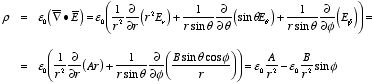
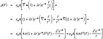
Example: Problem 2.46
Suppose the electric potential is
given by the expression
for all
r (
A and
λ are constants). Find the
electric field

,
the charge density

,
and the total charge
Q.
The electric field
can be immediately obtained from the electric potential:
The charge density
can be found using the electric field
and the following relation:
This expression shows that
Substituting the expression for the electric field
we obtain for the charge density
:
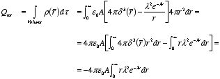
The total charge
Q can be found by volume integration of
:
The integral can be solved easily:
The total charge is thus equal to
The charge distribution
can be directly used to obtained from the electric potential

This equation can be rewritten as
and is known as
Poisson's equation. In the regions where

this equation reduces to
Laplace's equation:
The electric potential generated by a discrete charge distribution can be
obtained using the principle of superposition:
where

is the electric potential generated by the point charge

.
A point charge
located at the origin will generate an electric potential
equal to
In general, point charge
will be located at position

and the electric potential generated by this point charge at position

is equal to
The total electric potential generated by the whole set of point charges is
equal to
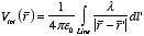
To calculate the electric potential generated by a continuous charge
distribution we have to replace the summation over point charges with an
integration over the continuous charge distribution. For the three charge
distributions we will be using in this course we obtain:
1. line charge
λ :
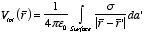
2. surface
charge
σ :
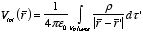
3. volume
charge
ρ :
 Example:
Problem 2.25
Example:
Problem 2.25 Using the general expression for
V in terms of
ρ find the potential at a distance
z above the center of the
charge distributions of Figure 2.8. In each case, compute

.
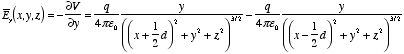
Suppose that we changed the right-hand charge in Figure 2.8a to -
q. What
is then the potential at
P? What field does this suggest? Compare your
answer to Problem 2.2b, and explain carefully any discrepancy.
 Figure
2.8. Problem 2.35.
Figure
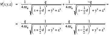
2.8. Problem 2.35.a) The electric potential at P generated by the two point charges is
equal to
The electric field generated by the two point charges can be obtained by
taking the gradient of the electric potential:
If we change the right-hand charge to -q then the total potential at
P is equal to zero. However, this does not imply that the electric field
at P is equal to zero. In our calculation we have assumed right from the
start that x = 0 and y = 0. Obviously, the potential at P
will therefore not show an x and y dependence. This however not
necessarily indicates that the components of the electric field along the
x and y direction are zero. This can be demonstrated by
calculating the general expression for the electric potential of this charge
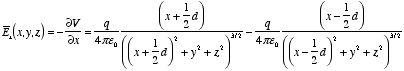
distribution at an arbitrary point (x,y,z):
The various components of the electric field can be obtained by taking the
gradient of this expression:
The components of the electric field at P = (0, 0, z) can now
be calculated easily:
b) Consider a small segment of the rod, centered at position
x and
with length
dx. The charge on this segment is equal to

.
The potential generated by this segment at
P is equal to
The total potential generated by the rod at P can be obtained by
integrating dV between x = - L and x =
L
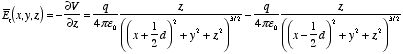
The z component of the electric field at P can be obtained
from the potential V by calculating the z component of the
gradient of V. We obtain
c) Consider a ring of radius r and width dr. The charge on
this ring is equal to
The electric potential dV at P generated by this ring is
equal to
The total electric potential at P can be obtained by integrating
dV between r = 0 and r = R:
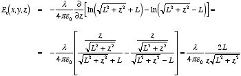
The z component of the electric field generated by this charge
distribution can be obtained by taking the gradient of V:
Example: Problem 2.5
Find the electric field a distance
z above the center of a circular loop of radius r, which carries a
uniform line charge λ.
The total charge Q on the ring is
equal to
The total electric potential V at P is equal to
The z component of the electric field at P can be obtained by
calculating the gradient of V:
This is the same answer we obtained in the beginning of this Chapter by
taking the vector sum of the segments of the ring.
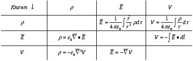
We have seen so far
that there are three fundamental quantities of electrostatics:
1. The
charge density ρ 2. The
electric field

3. The
electric potential VIf one of these quantities is known,
the others can be calculated:
In general the charge density
ρ and the electric field

do not have to be continuous. Consider for example an infinitesimal thin charge
sheet with surface charge
σ. The relation between the electric
field above and below the sheet can be obtained using Gauss's law. Consider a
rectangular box of height
ε and area
A (see Figure 2.9). The
electric flux through the surface of the box, in the limit
ε →
0, is equal to
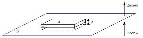 Figure
2.9. Electric field near a charge sheet.
Figure
2.9. Electric field near a charge sheet.where

and

are the perpendicular components of the electric field above and below the
charge sheet. Using Gauss's law and the rectangular box shown in Figure 2.9 as
integration volume we obtain
This equation shows that the electric field perpendicular to the charge
sheet is discontinuous at the boundary. The difference between the
perpendicular component of the electric field above and below the charge sheet
is equal to
The tangential component of the electric field is always continuous at any
boundary. This can be demonstrated by calculating the line integral of

around a rectangular loop of length
L and height
ε (see
Figure 2.10). The line integral of
,
in the limit
ε → 0, is equal to

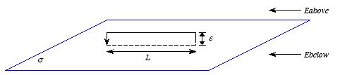 Figure
2.10. Parallel field close to charge sheet.
Figure
2.10. Parallel field close to charge sheet.Since the line integral of
around any closed loop is zero we conclude that
or
These boundary conditions for
can be combined into a single formula:
where

is a unit vector perpendicular to the surface and pointing towards the
above region.
The electric potential is continuous across any
boundary. This is a direct results of the definition of
V in terms of
the line integral of
:
If the path shrinks the line integral will approach zero, independent of
whether
is continuous or discontinuous. Thus
Example: Problem 2.30a) Check that the results of examples
4 and 5 of Griffiths are consistent with the boundary conditions for
.
b) Use
Gauss's law to find the field inside and outside a long hollow cylindrical tube
which carries a uniform surface charge
σ. Check that your results
are consistent with the boundary conditions for
.
c) Check
that the result of example 7 of Griffiths is consistent with the boundary
conditions for
V.
a)
Example 4 (Griffiths): The
electric field generated by an infinite plane carrying a uniform surface charge
σ is directed perpendicular to the sheet and has a magnitude equal
to
Therefore,
which is in agreement with the boundary conditions for
.
Example
5 (Griffiths): The electric field generated by the two charge sheets is
directed perpendicular to the sheets and has a magnitude equal to
The change in the strength of the electric field at the left sheet is equal
to
The change in the strength of the electric field at the right sheet is
equal to
These relations show agreement with the boundary conditions for
.
b) Consider
a Gaussian surface of length
L and radius
r. As a result of the
symmetry of the system, the electric field will be directed radially. The
electric flux through this Gaussian surface is therefore equal to the electric
flux through its curved surface which is equal to
The charge enclosed by the Gaussian surface is equal to zero when r
< R. Therefore
when r < R. When r > R the charge
enclosed by the Gaussian surface is equal to
The electric field for r > R, obtained using Gauss' law,
is equal to
The magnitude of the electric field just outside the cylinder, directed
radially, is equal to
The magnitude of the electric field just inside the cylinder is equal
to
Therefore,
which is consistent with the boundary conditions for
E.
c) Example 7 (Griffiths): the electric potential
just outside the charged spherical shell is equal to
The electric potential just inside the charged spherical shell is equal
to
These two equations show that the electric potential is continuous at the
boundary.
2.4. Work and Energy in Electrostatics
Consider a point charge q1 located at the origin. A
point charge q2 is moved from infinity to a point a distance
r2 from the origin. We will assume that the point charge
q1 remains fixed at the origin when point charge
q2 is moved. The force exerted by q1 on
q2 is equal to
where

is the electric field generated by
q1. In order to move
charge
q2 we will have to exert a force opposite to

.
Therefore, the total work that must be done to move
q2 from
infinity to
r2 is equal to
where

is the electric potential generated by
q1 at position
r2. Using the equation of
V for a point charge, the
work
W can be rewritten as
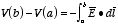
This work W is the work necessary to assemble the system of two
point charges and is also called the electrostatic potential
energy of the system. The energy of a system of more than two point
charges can be found in a similar manner using the superposition principle. For
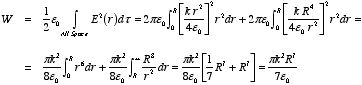
example, for a system consisting of three point charges (see Figure 2.11) the
electrostatic potential energy is equal to
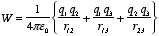
 Figure
2.11. System of three point charges.
Figure
2.11. System of three point charges.In this equation we have added the electrostatic energies of each pair of
point charges. The general expression of the electrostatic potential energy for
n point charges is
The lower limit of j (= i + 1) insures that each pair of
point charges is only counted once. The electrostatic potential energy can also
be written as
where Vi is the electrostatic potential at the location
of qi due to all other point charges.
When the charge of
the system is not distributed as point charges, but rather as a continuous
charge distribution ρ, then the electrostatic potential energy of
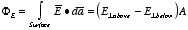
the system must be rewritten as
For continuous surface and line charges the electrostatic potential energy
is equal to
and
However, we have already seen in this Chapter that
ρ,
V,
and

carry the same equivalent information. The charge density
ρ, for
example, is related to the electric field
:
Using this relation we can rewrite the electrostatic potential energy
as
where we have used one of the product rules of vector derivatives and the
definition of
in terms of
V. In deriving this expression we have not made any
assumptions about the volume considered. This expression is therefore valid for
any volume. If we consider all space, then the contribution of the surface
integral approaches zero since

will approach zero faster than 1/
r2. Thus the total
electrostatic potential energy of the system is equal to

Example: Problem 2.45 A sphere of radius
R carries
a charge density

(where
k is a constant). Find the energy of the configuration. Check
your answer by calculating it in at least two different ways.
Method
1:
The first method we will use to calculate the electrostatic potential
energy of the charged sphere uses the volume integral of

to calculate
W. The electric field generated by the charged sphere can
be obtained using Gauss's law. We will use a concentric sphere of radius
r as the Gaussian surface. First consider the case in which
r
<
R. The charge enclosed by the Gaussian surface can be obtained by
volume integration of the charge distribution:
The electric flux through the Gaussian surface is equal to
Applying Gauss's law we find for the electric field inside the sphere
(r < R):
The electric field outside the sphere (r > R) can also be
obtained using Gauss's law:
The total electrostatic energy can be obtained from the electric
field:
Method 2:
An alternative way calculate the electrostatic
potential energy is to use the following relation:
The electrostatic potential
V can be obtained immediately from the
electric field

.
To evaluate the volume integral of

we only need to know the electrostatic potential
V inside the charged
sphere:
The electrostatic potential energy of the system is thus equal to
which is equal to the energy calculated using method 1.
2.5. Metallic Conductors
In a metallic conductor one or more electrons per atom are free to
move around through the material. Metallic conductors have the following
electrostatic properties:
1. The electric field inside the conductor
is equal to zero.
If there would be an electric field inside the
conductor, the free charges would move and produce an electric field of their
own opposite to the initial electric field. Free charges will continue to flow
until the cancellation of the initial field is complete.
2. The charge
density inside a conductor is equal to zero.
This property is a direct
result of property 1. If the electric field inside a conductor is equal to
zero, then the electric flux through any arbitrary closed surface inside the
conductor is equal to zero. This immediately implies that the charge density
inside the conductor is equal to zero everywhere (Gauss's law).
3. Any
net charge of a conductor resides on the surface.
Since the charge
density inside a conductor is equal to zero, any net charge can only reside on
the surface.
4. The electrostatic potential V is constant
throughout the conductor.
Consider two arbitrary points a and
b inside a conductor (see Figure 2.12). The potential difference between
a and b is equal to
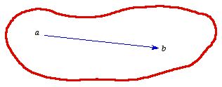 Figure
2.12. Potential inside metallic conductor.
Figure
2.12. Potential inside metallic conductor. Since the electric field inside a conductor is equal to zero, the line
integral of

between
a and
b is equal to zero. Thus
or
5. The electric field is perpendicular to the surface, just outside the
conductor.
If there would be a tangential component of the electric
field at the surface, then the surface charge would immediately flow around the
surface until it cancels this tangential component.
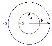
Example: A
spherical conducting shell
a) Suppose we place a point charge q at
the center of a neutral spherical conducting shell (see Figure 2.13). It will
attract negative charge to the inner surface of the conductor. How much induced
charge will accumulate here?
b) Find E and V as function of
r in the three regions r < a, a < r
< b, and r > b.
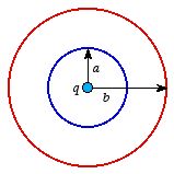 Figure
2.13. A spherical conducting shell.
Figure
2.13. A spherical conducting shell.a) The electric field inside the conducting shell is equal to zero
(property 1 of conductors). Therefore, the electric flux through any concentric
spherical Gaussian surface of radius
r (
a<
r<
b)
is equal to zero. However, according to Gauss's law this implies that the
charge enclosed by this surface is equal to zero. This can only be achieved if
the charge accumulated on the inside of the conducting shell is equal to
-
q. Since the conducting shell is neutral and any net charge must reside
on the surface, the charge on the outside of the conducting shell must be equal
to +
q.
b) The electric field generated by this system can be
calculated using Gauss's law. In the three different regions the electric field
is equal
to

for
b <
r 
for
a <
r <
b for
r <
aThe electrostatic potential
V(
r) can
be obtained by calculating the line integral of
from infinity to a point a distance
r from the origin. Taking the
reference point at infinity and setting the value of the electrostatic potential
to zero there we can calculate the electrostatic potential. The line integral
of
has to be evaluated for each of the three regions separately.
For
b
<
r:
For a < r < b:
For r < a:

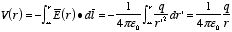
 Figure
2.14. Arbitrarily shaped conductor.
Figure
2.14. Arbitrarily shaped conductor.In this example we have looked at a symmetric system but the general
conclusions are also valid for an arbitrarily shaped conductor. For example,
consider the conductor with a cavity shown in Figure 2.14. Consider also a
Gaussian surface that completely surrounds the cavity (see for example the
dashed line in Figure 2.14). Since the electric field inside the conductor is
equal to zero, the electric flux through the Gaussian surface is equal to zero.
Gauss's law immediately implies that the charge enclosed by the surface is equal
to zero. Therefore, if there is a charge
q inside the cavity there will
be an induced charge equal to -
q on the walls of the cavity. On the
other hand, if there is no charge inside the cavity then there will be no charge
on the walls of the cavity. In this case, the electric field inside the cavity
will be equal to zero. This can be demonstrated by assuming that the electric
field inside the cavity is not equal to zero. In this case, there must be at
least one field line inside the cavity. Since field lines originate on a
positive charge and terminate on a negative charge, and since there is no charge
inside the cavity, this field line must start and end on the cavity walls (see
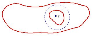
for example Figure 2.15). Now consider a closed loop, which follows the field
line inside the cavity and has an arbitrary shape inside the conductor (see
Figure 2.15). The line integral of
inside the cavity is definitely not equal to zero since the magnitude of
is not equal to zero and since the path is defined such that
and

are parallel. Since the electric field inside the conductor is equal to zero,
the path integral of
inside the conductor is equal to zero. Therefore, the path integral of
along the path indicated in Figure 2.15 is not equal to zero if the magnitude of
is not equal to zero inside the cavity. However, the line integral of
along any closed path must be equal to zero and consequently the electric field
inside the cavity must be equal to zero.
 Figure
2.15. Field line in cavity.
Figure
2.15. Field line in cavity.
Example: Problem 2.35
A metal sphere of radius R,
carrying charge q, is surrounded by a thick concentric metal shell (inner
radius a, outer radius b, see Figure 2.16). The shell carries no
net charge.
a) Find the surface charge density σ at R, at
a, and at b.
b) Find the potential at the center of the sphere,
using infinity as reference.
c) Now the outer surface is touched to a
grounding wire, which lowers its potential to zero (same as at infinity). How
do your answers to a) and b) change?
a) Since the net charge of a
conductor resides on its surface, the charge q of the metal sphere will
reside its surface. The charge density on this surface will therefore be equal
to
As a result of the charge on the metal sphere there will be a charge equal
to -q induced on the inner surface of the metal shell. Its surface
charge density will therefore be equal to
Since the metal shell is neutral there will be a charge equal to +q
on the outside of the shell. The surface charge density on the outside of the
shell will therefore be equal to

 Figure
2.16. Problem 2.35.
Figure
2.16. Problem 2.35.b) The potential at the center of the metal sphere can be found by
calculating the line integral of
between infinity and the center. The electric field in the regions outside the
sphere and shell can be found using Gauss's law. The electric field inside the
shell and sphere is equal to zero. Therefore,
c) When the outside of the shell is grounded, the charge density on the
outside will become zero. The charge density on the inside of the shell and on
the metal sphere will remain the same. The electric potential at the center of
the system will also change as a result of grounding the outer shell. Since the
electric potential of the outer shell is zero, we do not need to consider the
line integral of
in the region outside the shell to determine the potential at the center of the
sphere. Thus
Consider a conductor with surface charge σ, placed in an
external electric field. Because the electric field inside the conductor is
zero, the boundary conditions for the electric field require that the field
immediately above the conductor is equal to

 Figure
2.17. Patch of surface of conductor.
Figure
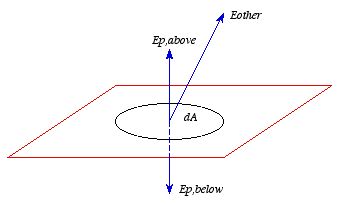
2.17. Patch of surface of conductor.This electric field will exert a force on the surface charge.
Consider
a small, infinitely thin, patch of the surface with surface area dA (see
Figure 2.17). The electric field directly above and below the patch is equal to
the vector sum of the electric field generated by the patch, the electric field
generated by the rest of the conductor and the external electric field. The
electric field generated by the patch is equal to
The remaining field,

,
is continuous across the patch, and consequently the total electric field above
and below the patch is equal to
These two equations show that
is equal to
In this case the electric field below the surface is equal to zero and the
electric field above the surface is directly determined by the boundary
condition for the electric field at the surface. Thus
Since the patch cannot exert a force on itself, the electric force exerted
on it is entirely due to the electric field
.
The charge on the patch is equal to

.
Therefore, the force exerted on the patch is equal to
The force per unit area of the conductor is equal to
This equation can be rewritten in terms of the electric field just outside
the conductor as
This force is directed outwards. It is called the radiation
pressure.
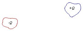
2.6. Capacitors
Consider two conductors (see Figure 2.18), one with a charge equal to
+Q and one with a charge equal to -Q. The potential difference
between the two conductors is equal to
Since the electric field

is proportional to the charge
Q, the potential difference ∆
V
will also be proportional to
Q. The constant of proportionality is
called the
capacitance C of the system and is defined as

 Figure
2.18. Two conductors.
Figure
2.18. Two conductors.The capacitance C is determined by the size, the shape, and the
separation distance of the two conductors. The unit of capacitance is the
farad (F). The capacitance of a system of conductors can in
general be calculated by carrying out the following steps:
1. Place a charge
+Q on one of the conductors. Place a charge of -Q on the other
conductor (for a two conductor system).
2. Calculate the electric field in
the region between the two conductors.
3. Use the electric field calculated
in step 2 to calculate the potential difference between the two
conductors.
4. Apply the result of part 3 to calculate the
capacitance:
We will now discuss two examples in which we follow these steps to
calculate the capacitance.
Example: Example 2.11
(Griffiths)
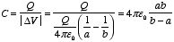
Find the capacitance of two concentric shells, with radii
a and b.
Place a charge +Q on the inner shell and a
charge -Q on the outer shell. The electric field between the shells can
be found using Gauss's law and is equal to
The potential difference between the outer shell and the inner shell is
equal to
The capacitance of this system is equal to
 Figure
2.19. Example 2.11.
Figure
2.19. Example 2.11. A system does not have to have two conductors in order to have a
capacitance. Consider for example a single spherical shell of radius R.
The capacitance of this system of conductors can be calculated by following the
same steps as in Example 12. First of all, put a charge Q on the
conductor. Gauss's law can be used to calculate the electric field generated by
this system with the following result:
Taking infinity as the reference point we can calculate the electrostatic
potential on the surface of the shell:
Therefore, the capacitance of the shell is equal to
Let us now consider a parallel-plate capacitor. The work required to
charge up the parallel-plate capacitor can be calculated in various
ways:
Method 1: Since we are free to chose the reference
point and reference value of the potential we will chose it such that the
potential of the positively charges plate is

and the potential of the negatively charged plate is

.
The energy of this charge distribution is then equal to
Method 2: Let us look at the charging process in detail.
Initially both conductors are uncharged and

.
At some intermediate step in the charging process the charge on the positively
charged conductor will be equal to
q. The potential difference between
the conductors will then be equal to
To increase the charge on the positively charged conductor by
dq we
have to move this charge
dq across this potential difference

.
The work required to do this is equal to
Therefore, the total work required to charge up the capacitor from q
= 0 to q = Q is equal to
Example: Problem 2.40.
Suppose the plates of a
parallel-plate capacitor move closer together by an infinitesimal distance
ε, as a result of their mutual attraction.
a) Use equation (2.45)
of Griffiths to express the amount of work done by electrostatic forces, in
terms of the field E and the area of the plates A.
b) Use
equation (2.40) of Griffiths to express the energy lost by the field in this
process.
a) We will assume that the parallel-plate capacitor is an ideal
capacitor with a homogeneous electric field E between the plates and no
electric field outside the plates. The electrostatic force per unit surface
area is equal to
The total force exerted on each plate is therefore equal to
As a result of this force, the plates of the parallel-plate capacitor move
closer together by an infinitesimal distance ε. The work done by
the electrostatic forces during this movement is equal to
b) The total energy stored in the electric field is equal to
In an ideal capacitor the electric field is constant between the plates and
consequently we can easily evaluate the volume integral of

:
where d is the distance between the plates. If the distance between
the plates is reduced, then the energy stored in the field will also be reduced.
A reduction in d of ε will reduce the energy stored by an
amount ∆W equal to
which is equal to the work done by the electrostatic forces on the
capacitor plates (see part a).